Transcription
J. Non-Newtonian Fluid Mech. xxx (2006) xxx–xxxFour-field Galerkin/least-squares formulation for viscoelastic fluidsOscar M. Coronado a , Dhruv Arora a , Marek Behr a,b, , Matteo Pasquali a, aDepartment of Chemical and Biomolecular Engineering and Computer and Information Technology Institute, Rice University,MS 362, 6100 Main Street, Houston, TX 77005, USAb Chair for Computational Analysis of Technical Systems, CCES, RWTH Aachen University, 52056 Aachen, GermanyReceived 4 November 2005; received in revised form 14 February 2006; accepted 24 March 2006AbstractA new Galerkin/Least-Squares (GLS) stabilized finite element method is presented for computing viscoelastic flows of complex fluids describedby the conformation tensor; it extends the well-established GLS method for computing flows of incompressible Newtonian fluids. GLS methodsare attractive for large-scale computations because they yield linear systems that can be solved easily with iterative solvers (e.g., the GeneralizedMinimum Residual method) and because they allow simple combinations of interpolation functions that can be conveniently and efficientlyimplemented on modern distributed-memory cache-based clusters.Like other state-of-the-art methods for computing viscoelastic flows (e.g., DEVSS-TG/SUPG), the new GLS method introduces a separate variableto represent the velocity gradient; with the aid of this variable, the conservation equations of mass, momentum, conformation, and the definitionof velocity gradient are converted into a set of first-order partial differential equations in four unknown fields—pressure, velocity, conformation,and velocity gradient. The unknown fields are represented by low-order (continuous piecewise linear or bilinear) finite element basis functions.The method is applied to the Oldroyd-B constitutive equation and is tested in two benchmark problems—flow in a planar channel and flowpast a cylinder in a channel. Results show that (1) the mesh-convergence rate of GLS is comparable to the DEVSS-TG/SUPG method; (2) the LSstabilization permits using equal-order basis functions for all fields; (3) GLS handles effectively the advective terms in the evolution equation ofthe conformation tensor; and (4) GLS yields accurate results at lower computational costs than DEVSS-type methods. 2006 Elsevier B.V. All rights reserved.Keywords: Stabilized finite element method; Viscoelastic flow; Galerkin/least-squares; Oldroyd-B fluid; Flow past a cylinder in a channel1. IntroductionIn the past decades, extensive research has been done on flowsof liquids with micro–macro structure (also known as complexfluids); these fluids are found in several industrial and biologicalapplications, e.g., polymer processing, coating of polymersolutions, ink-jet printing, microfluidic devices, and human aswell as artificial organs (blood, synovial fluid). Usually theseliquids display a viscosity dependent on the rate of strainingand the flow kinematics (shear versus extension); they alsoshow elasticity on time scales that overlap with the flow timescales.Realistic models of flowing complex fluids are crucial forunderstanding and optimizing flow processes. Two main classes Corresponding authors. Tel.: 1 713 348 5830; fax: 1 713 348 5478.E-mail address: mp@rice.edu (M. Pasquali), behr@cats.rwth-aachen.de(M. Behr).of models have been proposed for modeling complex fluids:fine-grained models [1,2], (e.g., bead-spring or bead-rod modelsof polymer solutions), where the microstructure is representedby micromechanical objects governed by stochastic differentialequations, and coarse-grained ones, where the microstructureis modeled by means of one or more continuum variables representing the expectation value of microscopic features (e.g.,the conformation tensor in models of polymer solutions) [3–6].Fine-grained models incorporate a richer degree of moleculardetails, but are still limited to fairly simple flows because ofcomputational cost [7–9].Coarse-grained models represent the liquid microstructurein terms of one or more conformation tensors; currently, thesemodels are considered the most appropriate for large-scale simulation of complex flows of complex fluids. Typically, the conformation tensor obeys a hyperbolic partial differential transportequation. In polymer solutions and melts, this tensor representsthe local expectation value of the polymer stretch and orientation, e.g., gyration or birefringence tensor. The elastic part0377-0257/ – see front matter 2006 Elsevier B.V. All rights ; No. of Pages 13
2O.M. Coronado et al. / J. Non-Newtonian Fluid Mech. xxx (2006) xxx–xxxof the stress is related to the conformation tensor through analgebraic equation [3–6]. Such models include most “classical”rate-type stress-based differential models (e.g., Oldroyd-B, PTT,Giesekus, etc.) [3–6].Simulations of complex flows of complex fluids requiresolving simultaneously the hyperbolic transport equation ofconformation (or rate-type equation for the stress) togetherwith the momentum and mass conservation equations; thisposes several numerical challenges. In particular, obtainingmesh-converged solutions in simple benchmark flows at highWeissenberg number (Wi, the product of characteristic strainrate and fluid relaxation time) is still considered an openproblem.The Galerkin method is perhaps the most effective methodfor flows with free surfaces and deformable boundaries. However, the Galerkin method is unstable in advection-dominatedproblems, and yields spurious oscillations in the variablefields. Alternative methods have been developed to handleadvection-dominated as well as purely hyperbolic equations—e.g., Streamline upwind/Petrov–Galerkin (SUPG) for highReynolds number Newtonian flows [10] and viscoelastic flows[11], also Discontinuous Galerkin (DG) for viscoelastic flows[12].When the Galerkin (or SUPG) method is applied to coupled partial differential equations, the selection of the interpolating functions for the various unknowns can be restricted bycompatibility conditions—e.g., the Babuška-Brezzi condition inflows of incompressible Newtonian fluids [13,14]. Some compatibility conditions between the basis functions of velocity,pressure, velocity gradient, and conformation (or stress) muststill be satisfied [15,16] by current Galerkin-type methods forsimulating viscoelastic flows—e.g., the state-of-the-art DEVSSTG/SUPG, which evolved from successive modifications of theEVSS method [17–22] (see also reviews by Baaijens [23] andOwens and Phillips [24]).These two key hurdles (handling advection-dominated problem and satisfying compatibility conditions) have been overcome in Newtonian flows by using Galerkin/Least-Squares(GLS) methods [25–27]. Work on GLS methods applied to Newtonian flows has shown that Streamline-upwind terms appearnaturally in the GLS form, that equal-order basis functions canbe used for all fields (because the Least-Squares (LS) terms remove the compatibility condition), and that the resulting nonlinear algebraic equations yield a Jacobian matrix that can be solvedmore easily with preconditioned Generalized Minimum Residual method (GMRES) (because the LS terms yield a positivedefinite Jacobian component). Moreover, using equal-order basis functions for all fields allows “nodal” (rather than “elemental”) accounting, which speeds up greatly matrix operations ondistributed memory parallel machines [28].Weakly consistent forms of GLS method have been applied toviscoelastic flows. Behr [25] introduced a three-field (velocity–pressure–elastic stress) GLS method and studied the flow ofan Oldroyd-B liquid in a 4-to-1 contraction. However, a detailedcomparison between this method and other published results wasnot performed, and the effect of the expression of the LS stabilization coefficient for the constitutive equation was not exam-ined. This method has been refined and extended more recentlyto improve consistency by recovery of the velocity gradient aswell as a more appropriate expression of the LS stabilizationcoefficient [29].Fan et al. [30] independently introduced an incomplete GLSmethod for viscoelastic flow and tested its performance in a flowbetween eccentric cylinders, flow around a sphere in a pipe, andflow around a cylinder in a channel. This method did not includeterms due to the LS form of the momentum equation (becauseit degraded performance) and of the constitutive equation;therefore, the method of Fan et al. [30] is better characterized asa pressure-stabilized SUPG method—see [31] for a descriptionof pressure-stabilized methods for incompressible Newtonianflows.This article presents a complete GLS method for computingflows of incompressible viscoelastic liquids modeled by conformation tensor or rate-type equations. The flow equations areconverted to a set of four first-order partial differential equations by representing explicitly the velocity gradient tensor (asin DEVSS-G). The GLS weighted residual equations includenaturally the consistent streamline upwinding for the advectiveterms in the conformation evolution equation (and in the momentum equation, although the presentation below is restrictedto inertialess flows). The choice of basis functions for the fourunknown fields (velocity, pressure, velocity gradient, and conformation) is not restricted by compatibility conditions; here,the unknown fields are represented by the simplest possible finite element basis functions—continuous piecewise bilinear onquadrilateral elements. The method is termed GLS4 to distinguish it from the previous GLS3 [25,29] method, in which thevelocity gradient was not represented explicitly. The accuracyand stability of the method is demonstrated by using two benchmark problems — the flow in a planar channel and the flow pasta cylinder in a channel — for an Oldroyd-B fluid.It is worth noting that recent work [32–34] identified anothersource of instability in low-order finite difference and finite element methods for computing viscoelastic flows—namely, theinability of low-order methods to capture exponentially growing profiles of conformation or elastic stress in regions of strongflow. Such instability can be avoided by using the logarithm ofthe conformation tensor as field variable [32], which has theadditional benefit of ensuring that the conformation tensor isautomatically positive definite everywhere in the flow. The proposed GLS4 method does not address this source of instabilityexplicitly. However, as discussed in Ref. [32], the logarithmicchange of variable is generally applicable to any finite elementmethod (see, e.g. [34]); thus, it should be possible to combine thecurrent GLS4 formulation with the log-conformation method toimprove the method further.2. Governing equationsThe steady flow of an inertialess incompressible viscoelastic fluid, occupying a spatial domain Ω, with boundary Γ isgoverned by the momentum and continuity equations: · T 0,on Ω,(1)
O.M. Coronado et al. / J. Non-Newtonian Fluid Mech. xxx (2006) xxx–xxx · v 0,on Ω,(2)where v is the liquid velocity and T is the stress tensor, whichcan be decomposed into a constitutively undetermined isotropiccontribution related to incompressibility, and viscous and elasticcontributions:T pI τ σ,(3)respectively, where p is the pressure, I the identity tensor, τ 2ηs D the viscous stress (usually due to solvent contribution), ηsthe solvent viscosity, and D is the rate-of-strain tensor, i.e., thesymmetric part of the velocity gradient. In order to transform theequations of motion into a set of first-order partial differentialequations (necessary for developing a consistent LS formulationfor low-order elements), an additional variable L is introducedto represent the velocity gradient:L v 1( · v)I,tr I(4)where tr denotes trace.The last term in Eq. (4) ensures that L remains traceless evenin the finite-precision solution [22]; with this definition, D (L LT )/2. In the Oldroyd-B model, the elastic stress is relatedto the dimensionless conformation tensor M through a simplelinear relationship σ G(M I), where G ηp /λ is the elasticmodulus, ηp the polymer contribution to the viscosity, and λ isthe relaxation time. The conformation tensor obeys a hyperbolicevolution equation: λM (M I) 0,(5) where M denotes an upper-convected derivative: TM v · M L · M M · L.(6)The equations governing the flow can be recast in dimensionlessform as: · T 0,(7) · v 0,(8)L v 1( · v )I 0,tr I Wi M (M I) 0,T p I β(L L T ) Boundary conditions on the momentum equation are neededon the entire boundary Γ Γg Γh . The essential and naturalboundary conditions are represented asv g(11)swhere β ηs η ηis the viscosity ratio. Hereafter, all variablespare dimensionless and the ( ) is omitted for clarity.(12)on Γh ,(13)where g and h are given functions, and n is the outward unitvector normal to the boundary. Because the equation of transport of conformation is hyperbolic, boundary conditions on theconformation tensor, represented by the tensor G, are imposedat inflow boundaries ΓG where v · n 0,M Gon ΓG .(14)3. Four-field Galerkin/least-squares formulation (GLS4)In this section, the GLS formulation of the governing equations (7)–(10) is presented. The method is termed GLS4 becausethe equation set has four basic unknown fields—v, p, L and M.The basis (interpolation) and weighting function spaces are:Shv {vh vh [H 1h (Ω)]nsd ,vh gh on Γg },(15)Vhv {vh vh [H 1h (Ω)]nsd ,vh 0 on Γg },(16)Shp Vhphh {p p H (Ω)},1h(17)ShL VhL {Lh Lh [H 1h (Ω)]nsd },2ShM {Mh Mh [H 1h (Ω)]ntc ,VhMhhntc {M M [H (Ω)] ,1hMh GhM 0(18)on ΓG },(19)on ΓG },(20)where H 1h represents functions with square integrable firstorder derivatives, nsd the number of spatial dimensions andntc nsd (nsd 1)/2 is the number of independent conformation tensor components. Bilinear piecewise continuous functions are used hereafter. The GLS4 formulation is: Find vh Svh ,h such that:p h Sph , Lh SLh and M h SMhhhh w : T dΩ w · h dΓΩ Ω Γh h 1 βhh Th τmom q β · (E (E ) ) Wi · S ·Ω [ · Th ] dΩ (10)1 β(M I),Wion Γg ,n·T h(9)where v v/vc , p p/(ηvc / lc ) and L L/(vc / lc ) are dimensionless velocity, pressure and interpolated traceless velocity gradient tensor, respectively. lc is the dimensionless gradient operator, vc is a characteristic velocity, and lc isa characteristic length. The dimensionless Weissenberg numberis Wi λ(vc / lc ). The dimensionless stress tensor T is3Ω ΩAqh ( · vh ) dΩτcont ( · wh )( · vh ) dΩEh : Lh vh 1( · vh )I dΩtr I 1( · wh )I : Lh vhtr IΩ 1( · vh )I dΩ Sh : Wi (vh · Mh (Lh )T · Mhtr IΩ Mh · Lh ) (Mh I) dΩ τcons Wi (vh · Sh τgradv Eh wh Ω
4O.M. Coronado et al. / J. Non-Newtonian Fluid Mech. xxx (2006) xxx–xxx (Lh )T · Sh Sh · Lh ) Sh : Wi (vh · Mh (Lh )T · Mh Mh · Lh ) (Mh I) dΩ 0, qh Vhp , wh Vhv , Eh VhL , Sh VhM ,(21)where τmom , τcont , τgradv and τcons are the LS stabilization parameters for the momentum, continuity, interpolated tracelessvelocity gradient and constitutive equations, respectively. Theunderbraced term A is neglected at low Wi because the (1/Wi)term grows large as Wi 0, causing numerical problems.3.1. Design of the stabilization coefficientsThe appropriate design of the four stabilization parameters —τmom , τcont , τgradv and τcons — in Eq. (21) plays a crucial role inthe performance of the method.The τmom -term stabilizes the Galerkin form in advectiondominated flows, and also removes the compatibility conditionbetween velocity and pressure spaces. The parameter designedspecifically for use with bilinear interpolations [31] is adaptedhere for the dimensionless system:τmom h2.4(22)where h is the dimensionless element length.The τcont -term improves the convergence of non-linearsolvers in advection-dominated problems. Hereafter, τcont 0because inertia is neglected.The τgradv -term stabilizes Eq. (4); although the associatedstabilization term is not strictly necessary, τgradv is taken here asτgradv 1.The τcons -term is introduced to stabilize the Galerkin format high Wi, and to bypass the compatibility conditions between velocity and conformation spaces. No systematic derivation for τcons is available in the literature. However, the transport equation of conformation can be viewed as an advection–generation equation, and considerable research has been doneon stabilization parameters for a simple advection–diffusion–generation equation [35–39]. Applying the definition proposedby Franca et al. [38], based on the convergence and stability analysis of advection-diffusion-generation equation, and extendedby Hauke [39], yieldsτcons1 1,Fig. 2. Mesh-convergence rate for a planar channel flow at different Wi. Theslope of the curves gives the rate of convergence with mesh refinement.Fig. 3. Geometry of a flow past a cylinder in a half channel.τcons2 1,Wi Lh (24)τcons3 h.2Wi vh (25)τcons1 and τcons2 are important in regions of the flow where generation is dominant, whereas τcons3 is important in advectiondominated regions. These three contributions can be combined(23)Fig. 1. Schematic of a flow in a planar channel with w/L 1/4. The top wallis kept fixed, the bottom wall is moving from right to left at v0 and a differentialpressure is applied between the left and right walls.Fig. 4. Flow past a cylinder in a channel, w/Rc 2: Finite element mesh M0(a) complete domain (b) detail of the mesh from x 2 to x 2.
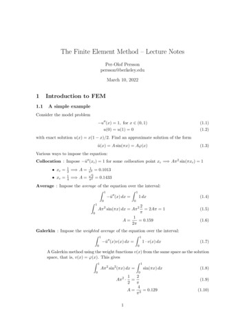
O.M. Coronado et al. / J. Non-Newtonian Fluid Mech. xxx (2006) xxx–xxxFig. 5. (Color online) Flow past a cylinder in a channel, w/Rc 2: drag forceon the cylinder versus Wi. The GLS4 results for the four meshes (M1, M2, M3and M4) are compared with the results presented by Sun et al. [21] and Hulsenet al. [34]. Inset: detail of the drag force at high Wi. 䊉 represents the drag forceon M4 at Wi 0.6. At Wi 0.6, the extrapolated value of the drag force is117.979, which is within 0.2% of the values reported in Refs. [30,34,40].as:τcons 1rτcons1 1rτcons2 1rτcons3 1/r,5Fig. 7. Flow past a cylinder in a channel, w/Rc 2: σxx on the cylinder and onthe symmetry line in the wake at Wi 0.7. from Hulsen et al. [34].(26)Hereafter, the switching parameter is set to r 2 (see alsoRef. [29]): 2 1/2h2Wi v τcons 1 (Wi Lh )2 .(27)h4. Numerical resultsThe proposed GLS4 formulation is tested in flow in a planar channel and flow past a cylinder in a channel. An analyticalsolution can be obtained in the former case; in the latter, theFig. 8. Flow past a cylinder in a channel, w/Rc 2: Drag force at Wi 0.6 forGLS4 and DEVSS-TG/SUPG for all meshes; dashed line represents the dragforce reported by Hulsen et al. [34] on their finest mesh.Fig. 6. Flow past a cylinder in a channel, w/Rc 2: σxx on the cylinder and onthe symmetry line in the wake at Wi 0.6. from Hulsen et al. [34].Fig. 9. Flow past a cylinder in a channel, w/Rc 2: Mesh-convergence rate ofthe drag force at Wi 0.6.
6O.M. Coronado et al. / J. Non-Newtonian Fluid Mech. xxx (2006) xxx–xxxcomputation of the relative errors e (numerical value analytical value)/(analytical value) 100% in region A. Fig. 2shows the maximum e in Myy (which has the highest e amongall unknown fields) versus the element size for Wi 3, 5 and 7.From the three curves the rate of mesh convergence is estimatedto be 1.73, 1.63 and 1.59, respectively. Because increase in Wiresults in increased generation, subsequently forming steeperboundary layer close to the channel walls, the rate of convergence is found to decrease. At Wi 3, Xie and Pasquali [41]reported a rate of convergence of 1.89 using DEVSS-TG/SUPGmethod with bi-quadratic interpolation for velocity.4.2. Flow past a cylinder in a channelFig. 10. Flow past a cylinder in a channel, w/Rc 2: Mesh-convergence rateof Mxx at a point in the wake flow (x 2; y 0) at Wi 0.6.numerical results from other state-of-the-art methods are usedfor validation [20–22,29,34,40]. The flow past a cylinder in achannel is a standard benchmark problem with desirable characteristics of smooth boundaries, and poses several numericalchallenges at high Wi due to the formation of sharp boundarylayers on the cylinder and in the wake.4.1. Flow in a planar channelFig. 1 shows a combination of Poiseuille flow (pushing liquid from left to right) and Couette flow (induced by the bottomwall dragging liquid from right to left with velocity v0 ) in a planar channel of width w 1 and length L 4w. The flow ofan Oldroyd-B fluid (β 0.59) is simulated, and the results arecompared with the known analytical solution. The figure alsoshows velocity profiles at the two open flow boundaries; bothright and left ends of the channel have respective inflow andoutflow sections. A region ‘A’ (dotted area in Fig. 1), which is2w in length and centrally placed in the channel, is monitoredfor comparing numerical results with analytical solution; thissufficiently eliminates the influences due to the boundary conditions. The problem setup closely follows the numerical exampleemployed by Xie and Pasquali [41]; the analytical solution forvelocity and conformation fields are p w y 2yyvx 1 v0 , vy 0, (28)2 Lwww dvx 2dvx, Myy 1, (29), Mxy λMxx 1 2 λdydywhere p 50 is the differential pressure between the leftand right boundaries. Consequently, Wi λ[ pw/(2L) 1](v0 /w). The Dirichlet conditions are imposed for velocity components on all boundaries, and the conformation tensor components are only specified at the corresponding inflows. The numerical results are obtainedon four different uniform meshes — 16 16, 24 24,32 32 and 64 64 — followed by a node-by-nodeThe flow of an Oldroyd-B fluid past a cylinder in a rectangular channel has been used as a standard benchmark problem totest several computational methods [20–22,29,34,40]. For computational ease, the symmetry of the problem is used and onlyhalf of the channel is simulated. Fig. 3 shows the schematic ofthe problem, where Lu , Ld , Rc and w represent the upstreamlength, the downstream length, the cylinder radius, and the halfchannel width, respectively.A no-slip boundary condition is imposed on the cylinder surface and channel walls, and fully developed flow conditions areassumed at the inflow and outflow boundaries. Consequently: Qy2vy 0,vx 1.51 2 ,(30)wwMxxQ y 3 λ 2 ,w wMyy 1, Mxy Myx3Qλy 1 2 3w 2,(31)where Q is the flow rate. Whereas the velocity is imposed atboth inflow and outflow, the conformation tensor componentsare specified at the inflow only. At the symmetry line, n · T 0and vy 0, where n is the unit vector normal to the symmetryline. The computed drag on the cylinder fd has been traditionallyused to compare numerical methods: (32)fd 2 e1 n : T dS,Swhere S represents the surface of the cylinder, n the unit normalvector, and e1 is the unit vector in the x-direction.4.2.1. Flow past a cylinder in a channel: w/Rc 2In this case, w 2, Rc 1, Lu 20, Ld 20, Q 2 andβ 0.59. Fig. 4 shows the mesh M0 from which four systematically refined meshes are obtained; in these meshes, the elementsare concentrated on the cylinder surface and in the wake alongthe symmetry line. The M1, M2, M3 and M4 meshes are obtained by dividing every element side of M0 by 3, 4, 5 and 6,respectively. The number of elements and corresponding number of unknowns are listed in Table 1. This flow problem posesnumerical challenges at high Wi; therefore, the maximum Wi upto which the numerical schemes converge has been employedas a measure of robustness (but not necessarily accuracy). For
O.M. Coronado et al. / J. Non-Newtonian Fluid Mech. xxx (2006) xxx–xxx7Fig. 11. (Color online) Flow past a cylinder in a channel, w/Rc 2: (a) Mxx , (b) Mxy and (c) Myy contours at Wi 0.7 on mesh M2.example, using DEVSS-G/SUPG, Sun et al. [21] reported solutions up to Wi 1.85, Fan et al. [30] using an incomplete GLSup to Wi 1.05 and Hulsen et al. [34] using the log conformation up to Wi 2.0; however, the accuracy of the solutions atWi 0.6 was not confirmed in these works.Here, a sequence of flow states is computed by first-orderarc-length continuation on Wi with automatic step control; thecontinuation terminates when the conformation tensor loses itspositive-definiteness, which occurs at Wi 0.7. The positivedefiniteness of M was not usually considered in past stud-Fig. 12. Flow past a cylinder in a channel, w/Rc 2: Mxx along line x 2 onmesh M3. Inset: detail of Mxx near the centerline (y 0).Fig. 13. Flow past a cylinder in a channel, w/Rc 2: Mxy along line x 2 onmesh M3. Inset: detail of Mxy near the centerline (y 0).
8O.M. Coronado et al. / J. Non-Newtonian Fluid Mech. xxx (2006) xxx–xxxFig. 14. Flow past a cylinder in a channel, w/Rc 2: Myy along line x 2 forM3. Inset: detail of Myy near the centerline (y 0).ies, with exception of the recent work of Hulsen et al. [34].Fig. 5 shows the drag forces on the meshes M1, M2 andM3; a good agreement is found up to Wi 0.4 with the results reported by Hulsen et al. [34] and Sun et al. [21]. Beyond that, the three methods show slight differences in thedrag predictions, while following the same trend. Figs. 6 and7 show σxx versus s at Wi 0.6 and 0.7, respectively, whereσxx (ηp /λ)Mxx and s is defined as: 0 s πRc on the cylinder and πRc s πRc Ld Rc in the wake along the symmetry line. At Wi 0.6, a complete overlap is observed amongthe results on the meshes M1, M2 and M3. In Fig. 6, σxx profiles computed with M1, M2 and M3 are overlapping in thewake; however, the result from M1 shows underprediction onthe cylinder, implying that refinement of M1 is not sufficient tocapture the steep boundary layer on the cylinder. On the otherhand, in Fig. 7, differences are observed not only on the cylinder but also in the wake flow. The figures also show the results reported by Hulsen et al. [34] at the corresponding Wi,Fig. 15. Flow past a cylinder in a channel, w/Rc 2: σxx on the cylinder andon the symmetry line at Wi 0.6. The GLS4 and DEVSS-TG/SUPG results areobtained for M2. from Hulsen et al. [34].Fig. 16. (Color online) Direct comparison of GLS4 and DEVSS-TG/SUPG withrespect to the number of elements (bottom axis) and to the number of degrees offreedom for conformation (top axis). The left and right axes represent the timeper Newton iteration (s) and memory usage (MB), respectively. A frontal solveris used in both simulations.Fig. 17. Flow past a cylinder in a channel, w/Rc 8: Finite element mesh M0(a) complete domain (b) detail of the mesh from x 4 to x 4.Fig. 18. Flow past a cylinder in a channel, w/Rc 8: Drag force on the threemeshes. The dotted curve is obtained from Sun et al. [21]. Inset: detail of thedrag force at high Wi.
O.M. Coronado et al. / J. Non-Newtonian Fluid Mech. xxx (2006) xxx–xxx9Fig. 19. (Color online) Flow past a cylinder in a channel, w/Rc 8: (a) Mxx , (b) Mxy and (c) Myy contours at Wi 2.0 on mesh M2.Table 1Flow past a cylinder in a channel, w/Rc 2: Characteristics of the finite element UnknownsTime per Newton iteration (s)GLS4DEVSSGLS4DEVSS 4996087890136460195670 79102139514216950311410 22064814602914 3229342144 Memory usage (MB)d 31.730.631.9 GLS4DEVSS 608141027204650 114026475122 d 46.746.746.9 is the % relative difference in the respective values from DEVSS and GLS4.Table 2Flow past a cylinder in a channel, w/Rc 8: Characteristics of the finite element meshesMeshElementsUnknownsTime per Newton iteration (s)Memory usage (MB)M0M1M2M32504000625012250 4169064610125450 1984401505 3968631859
10O.M. Coronado et al. / J. Non-Newtonian Fluid Mech. xxx (2006) xxx–xxxand good agreement is found with results on M3. In previousworks, the convergence of the stresses has been shown by comparing stress profiles obtained on systematically refined meshesusing p- and h-refinement [30,34]. While overlap of the resultsdemonstrates qualitatively mesh convergence, here, accuracy ismeasured more precisely by Richardson extrapolation:fd (h) fd (0) αhn ,(33)where fd (0) is the drag for an infinitely refined mesh, n the rate ofmesh convergence and α is a constant. fd (0) is used to computethe relative errors e (fd (h) fd (0))/fd (0) 100% in fd (h).Fig. 8 shows fd predictions from GLS4 and DEVSS-TG/SUPGalong with the results presented by Hulsen et al. [34] at Wi 0.6.The extrapolated values of fd for an infinitely refined meshare 117.979 and 117.778 for GSL4 and DEVSS-TG/SUPG,respectively. Thus, the GLS4 extrapolated results are within0.2% of the values computed by high resolution finite volume(fd 117.79 [40]), by pressure-stabilized finite elements (fd 117.78 [30]), by DEVSS-DG-Log conformation finite elements(fd 117.77 [34]), and by DEVSS-TG/SUPG calculations.Fig. 9 shows e versus h, and a mesh convergence rate of 2.39 isobserved.Similarly, Richardson extrapolation analysis is also performed for Mxx at a point in the wake flow (x 2; y 0).The extrapolated value of Mxx is 26.05 and the rate of meshconvergence is 1.74. Fig. 10 shows e versus h for Mxx . Inall cases, results on M4 are also employed to obtain the extrapolated values. Fig. 11 shows the conformation contours atWi 0.7, in which, the formation of sharp boundary layers onthe cylinder and along the symmetry line in the wake flow areobserved. These boundary layers are difficult to resolve numerically, and the onset of oscillations in the conformation fields isobserved as the boundary layers grow at high Wi. The influenceof the sharp boundary layer at high Wi is shown in Figs. 12–14, which plot M components along line x 2. At Wi 0.5and 0.6 a smooth profile for the M components is observed,whereas at Wi 0.7 oscillations appear towards the symmetry line (y 0). The m
Realistic models of flowing complex fluids are crucial for understanding and optimizing flow processes. Two main classes Corresponding authors. Tel.: 1 713 348 5830; fax: 1 713 348 5478. E-mail address: mp@rice.edu (M. Pasquali), behr@cats.rwth-aachen.de (M. Behr). of models have been proposed for modeling complex fluids: