Transcription
iLecture Notes on OptimizationPravin Varaiya
ii
Contents1 INTRODUCTION12 OPTIMIZATION OVER AN OPEN SET73 Optimization with equality constraints154 Linear Programming275 Nonlinear Programming496 Discrete-time optimal control757 Continuous-time linear optimal control838 Coninuous-time optimal control959 Dynamic programing121iii
ivCONTENTS
PREFACE to this editionNotes on Optimization was published in 1971 as part of the Van Nostrand Reinhold Notes on System Sciences, edited by George L. Turin. Our aim was to publish short, accessible treatments ofgraduate-level material in inexpensive books (the price of a book in the series was about five dollars). The effort was successful for several years. Van Nostrand Reinhold was then purchased by aconglomerate which cancelled Notes on System Sciences because it was not sufficiently profitable.Books have since become expensive. However, the World Wide Web has again made it possible topublish cheaply.Notes on Optimization has been out of print for 20 years. However, several people have beenusing it as a text or as a reference in a course. They have urged me to re-publish it. The idea ofmaking it freely available over the Web was attractive because it reaffirmed the original aim. Theonly obstacle was to retype the manuscript in LaTex. I thank Kate Klohe for doing just that.I would appreciate knowing if you find any mistakes in the book, or if you have suggestions for(small) changes that would improve it.Berkeley, CaliforniaSeptember, 1998P.P. Varaiyav
viCONTENTS
PREFACEThese Notes were developed for a ten-week course I have taught for the past three years to first-yeargraduate students of the University of California at Berkeley. My objective has been to present,in a compact and unified manner, the main concepts and techniques of mathematical programmingand optimal control to students having diverse technical backgrounds. A reasonable knowledge ofadvanced calculus (up to the Implicit Function Theorem), linear algebra (linear independence, basis,matrix inverse), and linear differential equations (transition matrix, adjoint solution) is sufficient forthe reader to follow the Notes.The treatment of the topics presented here is deep. Although the coverage is not encyclopedic,an understanding of this material should enable the reader to follow much of the recent technicalliterature on nonlinear programming, (deterministic) optimal control, and mathematical economics.The examples and exercises given in the text form an integral part of the Notes and most readers willneed to attend to them before continuing further. To facilitate the use of these Notes as a textbook,I have incurred the cost of some repetition in order to make almost all chapters self-contained.However, Chapter V must be read before Chapter VI, and Chapter VII before Chapter VIII.The selection of topics, as well as their presentation, has been influenced by many of my studentsand colleagues, who have read and criticized earlier drafts. I would especially like to acknowledgethe help of Professors M. Athans, A. Cohen, C.A. Desoer, J-P. Jacob, E. Polak, and Mr. M. Ripper. Ialso want to thank Mrs. Billie Vrtiak for her marvelous typing in spite of starting from a not terriblylegible handwritten manuscript. Finally, I want to thank Professor G.L. Turin for his encouragingand patient editorship.Berkeley, CaliforniaNovember, 1971P.P. Varaiyavii
viiiCONTENTS
Chapter 1INTRODUCTIONIn this chapter, we present our model of the optimal decision-making problem, illustrate decisionmaking situations by a few examples, and briefly introduce two more general models which wecannot discuss further in these Notes.1.1 The Optimal Decision ProblemThese Notes show how to arrive at an optimal decision assuming that complete information is given.The phrase complete information is given means that the following requirements are met:1. The set of all permissible decisions is known, and2. The cost of each decision is known.When these conditions are satisfied, the decisions can be ranked according to whether they incurgreater or lesser cost. An optimal decision is then any decision which incurs the least cost amongthe set of permissible decisions.In order to model a decision-making situation in mathematical terms, certain further requirementsmust be satisfied, namely,1. The set of all decisions can be adequately represented as a subset of a vector space with eachvector representing a decision, and2. The cost corresponding to these decisions is given by a real-valued function.Some illustrations will help.Example 1: The Pot Company (Potco) manufacturers a smoking blend called Acapulco Gold.The blend is made up of tobacco and mary-john leaves. For legal reasons the fraction α of maryjohn in the mixture must satisfy 0 α 12 . From extensive market research Potco has determinedtheir expected volume of sales as a function of α and the selling price p. Furthermore, tobacco canbe purchased at a fixed price, whereas the cost of mary-john is a function of the amount purchased.If Potco wants to maximize its profits, how much mary-john and tobacco should it purchase, andwhat price p should it set?Example 2: Tough University provides “quality” education to undergraduate and graduate students. In an agreement signed with Tough’s undergraduates and graduates (TUGs), “quality” is1
CHAPTER 1. INTRODUCTION2defined as follows: every year, each u (undergraduate) must take eight courses, one of which is aseminar and the rest of which are lecture courses, whereas each g (graduate) must take two seminarsand five lecture courses. A seminar cannot have more than 20 students and a lecture course cannothave more than 40 students. The University has a faculty of 1000. The Weary Old Radicals (WORs)have a contract with the University which stipulates that every junior faculty member (there are 750of these) shall be required to teach six lecture courses and two seminars each year, whereas everysenior faculty member (there are 250 of these) shall teach three lecture courses and three seminarseach year. The Regents of Touch rate Tough’s President at α points per u and β points per g “processed” by the University. Subject to the agreements with the TUGs and WORs how many u’s andg’s should the President admit to maximize his rating?Example 3: (See Figure 1.1.) An engineer is asked to construct a road (broken line) connectionpoint a to point b. The current profile of the ground is given by the solid line. The only requirementis that the final road should not have a slope exceeding 0.001. If it costs c per cubic foot to excavateor fill the ground, how should he design the road to meet the specifications at minimum cost?Example 4: Mr. Shell is the manager of an economy which produces one output, wine. Thereare two factors of production, capital and labor. If K(t) and L(t) respectively are the capital stockused and the labor employed at time t, then the rate of output of wine W (t) at time is given by theproduction functionW (t) F (K(t), L(t))As Manager, Mr. Shell allocates some of the output rate W (t) to the consumption rate C(t), andthe remainder I(t) to investment in capital goods. (Obviously, W , C, I, and K are being measuredin a common currency.) Thus, W (t) C(t) I(t) (1 s(t))W (t) where s(t) I(t)/W (t).ab.Figure 1.1: Admissable set of example. [0, 1] is the fraction of output which is saved and invested. Suppose that the capital stock decaysexponentially with time at a rate δ 0, so that the net rate of growth of capital is given by thefollowing equation:dK(t)dt δK(t) s(t)W (t)K̇(t) δK(t) s(t)F (K(t), L(t)).The labor force is growing at a constant birth rate of β 0. Hence,(1.1)
1.1. THE OPTIMAL DECISION PROBLEM3L̇(t) βL(t).(1.2)Suppose that the production function F exhibits constant returns to scale, i.e., F (λK, λL) λF (K, L) for all λ 0. If we define the relevant variable in terms of per capita of labor, w W/L, c C/L, k K/l, and if we let f (k) F (k, l), then we see that F (K, L) LF (K/L, 1) Lf (k), whence the consumption per capita of labor becomes c(t) (l s(t))f (k(t)). Using thesedefinitions and equations (1.1) and (1.2) it is easy to see that K(t) satisfies the differential equation(1.3).k̇(t) s(t)f (k(t)) µk(t)(1.3)where µ (δ β). The first term of the right-hand side in (3) is the increase in the capital-to-laborratio due to investment whereas the second terms is the decrease due to depreciation and increase inthe labor force.Suppose there is a planning horizon time T , and at time 0 Mr. Shell starts with capital-to-laborRTratio ko . If “welfare” over the planning period [0, T ] is identified with total consumption 0 c(t)dt,what should Mr. Shell’s savings policy s(t), 0 t T , be so as to maximize welfare? Whatsavings policy maximizes welfare subject to the additional restriction that the capital-to-labor ratioat time T should be at least kT ? If futureR consumption is discounted at rate α 0 and if time horizonis , the welfare function becomes 0 e αt c(t)dt. What is the optimum policy corresponding tothis criterion?These examples illustrate the kinds of decision-making problems which can be formulated mathematically so as to be amenable to solutions by the theory presented in these Notes. We must alwaysremember that a mathematical formulation is inevitably an abstraction and the gain in precision mayhave occurred at a great loss of realism. For instance, Example 2 is caricature (see also a faintly related but more more elaborate formulation in Bruno [1970]), whereas Example 4 is light-years awayfrom reality. In the latter case, the value of the mathematical exercise is greater the more insensitiveare the optimum savings policies with respect to the simplifying assumptions of the mathematicalmodel. (In connection with this example and related models see the critique by Koopmans [1967].)In the examples above, the set of permissible decisions is represented by the set of all pointsin some vector space which satisfy certain constraints. Thus, in the first example, a permissibledecision is any two-dimensional vector (α, p) satisfying the constraints 0 α 12 and 0 p. In the second example, any vector (u, g) with u 0, g 0, constrained by the numberof faculty and the agreements with the TUGs and WORs is a permissible decision. In the lastexample, a permissible decision is any real-valued function s(t), 0 t T , constrained by0 s(t) 1. (It is of mathematical but not conceptual interest to note that in this case a decisionis represented by a vector in a function space which is infinite-dimensional.) More concisely then,these Notes are concerned with optimizing (i.e. maximizing or minimizing) a real-valued functionover a vector space subject to constraints. The constraints themselves are presented in terms offunctional inequalities or equalities.
4CHAPTER 1. INTRODUCTIONAt this point, it is important to realize that the distinction between the function which is to beoptimized and the functions which describe the constraints, although convenient for presenting themathematical theory, may be quite artificial in practice. For instance, suppose we have to choosethe durations of various traffic lights in a section of a city so as to achieve optimum traffic flow.Let us suppose that we know the transportation needs of all the people in this section. Before wecan begin to suggest a design, we need a criterion to determine what is meant by “optimum trafficflow.” More abstractly, we need a criterion by which we can compare different decisions, which inthis case are different patterns of traffic-light durations. One way of doing this is to assign as cost toeach decision the total amount of time taken to make all the trips within this section. An alternativeand equally plausible goal may be to minimize the maximum waiting time (that is the total timespent at stop lights) in each trip. Now it may happen that these two objective functions may beinconsistent in the sense that they may give rise to different orderings of the permissible decisions.Indeed, it may be the case that the optimum decision according to the first criterion may be lead tovery long waiting times for a few trips, so that this decision is far from optimum according to thesecond criterion. We can then redefine the problem as minimizing the first cost function (total timefor trips) subject to the constraint that the waiting time for any trip is less than some reasonablebound (say one minute). In this way, the second goal (minimum waiting time) has been modifiedand reintroduced as a constraint. This interchangeability of goal and constraints also appears at adeeper level in much of the mathematical theory. We will see that in most of the results the objectivefunction and the functions describing the constraints are treated in the same manner.1.2 Some Other Models of Decision ProblemsOur model of a single decision-maker with complete information can be generalized along twovery important directions. In the first place, the hypothesis of complete information can be relaxedby allowing that decision-making occurs in an uncertain environment. In the second place, wecan replace the single decision-maker by a group of two or more agents whose collective decisiondetermines the outcome. Since we cannot study these more general models in these Notes, wemerely point out here some situations where such models arise naturally and give some references.1.2.1 Optimization under uncertainty.A person wants to invest 1,000 in the stock market. He wants to maximize his capital gains, andat the same time minimize the risk of losing his money. The two objectives are incompatible, sincethe stock which is likely to have higher gains is also likely to involve greater risk. The situationis different from our previous examples in that the outcome (future stock prices) is uncertain. It iscustomary to model this uncertainty stochastically. Thus, the investor may assign probability 0.5 tothe event that the price of shares in Glamor company increases by 100, probability 0.25 that theprice is unchanged, and probability 0.25 that it drops by 100. A similar model is made for all theother stocks that the investor is willing to consider, and a decision problem can be formulated asfollows. How should 1,000 be invested so as to maximize the expected value of the capital gainssubject to the constraint that the probability of losing more than 100 is less than 0.1?As another example, consider the design of a controller for a chemical process where the decisionvariable are temperature, input rates of various chemicals, etc. Usually there are impurities in thechemicals and disturbances in the heating process which may be regarded as additional inputs of a
1.2. SOME OTHER MODELS OF DECISION PROBLEMS5random nature and modeled as stochastic processes. After this, just as in the case of the portfolioselection problem, we can formulate a decision problem in such a way as to take into account theserandom disturbances.If the uncertainties are modelled stochastically as in the example above, then in many casesthe techniques presented in these Notes can be usefully applied to the resulting optimal decisionproblem. To do justice to these decision-making situations, however, it is necessary to give greatattention to the various ways in which the uncertainties can be modelled mathematically. We alsoneed to worry about finding equivalent but simpler formulations. For instance, it is of great significance to know that, given appropriate conditions, an optimal decision problem under uncertaintyis equivalent to another optimal decision problem under complete information. (This result, knownas the Certainty-Equivalence principle in economics has been extended and baptized the SeparationTheorem in the control literature. See Wonham [1968].) Unfortunately, to be able to deal withthese models, we need a good background in Statistics and Probability Theory besides the materialpresented in these Notes. We can only refer the reader to the extensive literature on Statistical Decision Theory (Savage [1954], Blackwell and Girshick [1954]) and on Stochastic Optimal Control(Meditch [1969], Kushner [1971]).1.2.2 The case of more than one decision-maker.Agent Alpha is chasing agent Beta. The place is a large circular field. Alpha is driving a fast, heavycar which does not maneuver easily, whereas Beta is riding a motor scooter, slow but with goodmaneuverability. What should Alpha do to get as close to Beta as possible? What should Betado to stay out of Alpha’s reach? This situation is fundamentally different from those discussed sofar. Here there are two decision-makers with opposing objectives. Each agent does not know whatthe other is planning to do, yet the effectiveness of his decision depends crucially upon the other’sdecision, so that optimality cannot be defined as we did earlier. We need a new concept of rational(optimal) decision-making. Situations such as these have been studied extensively and an elaboratestructure, known as the Theory of Games, exists which describes and prescribes behavior in thesesituations. Although the practical impact of this theory is not great, it has proved to be among themost fruitful sources of unifying analytical concepts in the social sciences, notably economics andpolitical science. The best single source for Game Theory is still Luce and Raiffa [1957], whereasthe mathematical content of the theory is concisely displayed in Owen [1968]. The control theoristwill probably be most interested in Isaacs [1965], and Blaquiere, et al., [1969].The difficulty caused by the lack of knowledge of the actions of the other decision-making agentsarises even if all the agents have the same objective, since a particular decision taken by our agentmay be better or worse than another decision depending upon the (unknown) decisions taken by theother agents. It is of crucial importance to invent schemes to coordinate the actions of the individualdecision-makers in a consistent manner. Although problems involving many decision-makers arepresent in any system of large size, the number of results available is pitifully small. (See Mesarovic,et al., [1970] and Marschak and Radner [1971].) In the author’s opinion, these problems representone of the most important and challenging areas of research in decision theory.
6CHAPTER 1. INTRODUCTION
Chapter 2OPTIMIZATION OVER AN OPENSETIn this chapter we study in detail the first example of Chapter 1. We first establish some notationwhich will be in force throughout these Notes. Then we study our example. This will generalizeto a canonical problem, the properties of whose solution are stated as a theorem. Some additionalproperties are mentioned in the last section.2.1 Notation2.1.1All vectors are column vectors, with two consistent exceptions mentioned in 2.1.3 and 2.1.5 belowand some other minor and convenient exceptions in the text. Prime denotes transpose so that ifx Rn then x0 is the row vector x0 (x1 , . . . , xn ), and x (x1 , . . . , xn )0 . Vectors are normallydenoted by lower case letters, the ith component of a vector x Rn is denoted xi , and differentvectors denoted by the same symbol are distinguished by superscripts as in xj and xk . 0 denotesboth the zero vector and the real number zero, but no confusion will result.Thus if x (x1 , . . . , xn )0 and y (y1 , . . . , yn )0 then x0 y x1 y1 . . . xn yn as in ordinarymatrix multiplication. If x Rn we define x x0 x.2.1.2If x (x1 , . . . , xn )0 and y (y1 , . . . , yn )0 then x y means xi yi , i 1, . . . , n. In particular ifx Rn , then x 0, if xi 0, i 1, . . . , n.2.1.3Matrices are normally denoted by capital letters. If A is an m n matrix, then Aj denotes the jthcolumn of A, and Ai denotes the ith row of A. Note that Ai is a row vector. Aji denotes the entryof A in the ith row and jth column; this entry is sometimes also denoted by the lower case letteraij , and then we also write A {aij }. I denotes the identity matrix; its size will be clear from thecontext. If confusion is likely, we write In to denote the n n identity matrix.7
CHAPTER 2. OPTIMIZATION OVER AN OPEN SET82.1.4If f : Rn Rm is a function, its ith component is written fi , i 1, . . . , m. Note that fi : Rn R.Sometimes we describe a function by specifying a rule to calculate f (x) for every x. In this casewe write f : x 7 f (x). For example, if A is an m n matrix, we can write F : x 7 Ax to denotethe function f : Rn Rm whose value at a point x Rn is Ax.2.1.5If f : Rn 7 R is a differentiable function, the derivative of f at x̂ is the row vector (( f / x1 )(x̂), . . . , ( f / xn )(x̂)).This derivative is denoted by ( f / x)(x̂) or fx (x̂) or f / x x x̂ or fx x x̂ , and if the argument x̂is clear from the context it may be dropped. The column vector (fx (x̂))0 is also denoted x f (x̂),and is called the gradient of f at x̂. If f : (x, y) 7 f (x, y) is a differentiable function fromRn Rm into R, the partial derivative of f with respect to x at the point (x̂, ŷ) is the n-dimensionalrow vector fx (x̂, ŷ) ( f / x)(x̂, ŷ) (( f / x1 )(x̂, ŷ), . . . , ( f / xn )(x̂, ŷ)), and similarlyfy (x̂, ŷ) ( f / y)(x̂, ŷ) (( f / y1 )(x̂, ŷ), . . . , ( f / ym )(x̂, ŷ)). Finally, if f : Rn Rm isa differentiable function with components f1 , . . . , fm , then its derivative at x̂ is the m n matrix f1x (x̂) f .(x̂) fx x̂ . xfmx (x̂) f1(x̂) . . . x1. . fm(x̂) x1 f1 xn (x̂). fm xn (x̂) 2.1.6If f : Rn R is twice differentiable, its second derivative at x̂ is the n n matrix ( 2 f / x x)(x̂) fxx (x̂) where (fxx (x̂))ji ( 2 f / xj xi )(x̂). Thus, in terms of the notation in Section 2.1.5 above,fxx (x̂) ( / x)(fx )0 (x̂).2.2 ExampleWe consider in detail the first example of Chapter 1. Define the following variables and functions:α fraction of mary-john in proposed mixture,p sale price per pound of mixture,v total amount of mixture produced,f (α, p) expected sales volume (as determined by market research) of mixture as a function of(α, p).
2.2. EXAMPLE9Since it is not profitable to produce more than can be sold we must have:v f (α, p),m amount (in pounds) of mary-john purchased, andt amount (in pounds) of tobacco purchased.Evidently,m αv, andt (l α)v.LetP1 (m) purchase price of m pounds of mary-john, andP2 purchase price per pound of tobacco.Then the total cost as a function of α, p isC(α, p) P1 (αf (α, p)) P2 (1 α)f (α, p).The revenue isR(α, p) pf (α, p),so that the net profit isN (α, p) R(α, p) C(α, p).The set of admissible decisions is Ω, where Ω {(α, p) 0 α 12 , 0 p }. Formally, wehave the the following decision problem:Maximize N (α, p),subject to (α, p) Ω.Suppose that (α , p ) is an optimal decision, i.e.,(α , p ) ΩandN (α , p ) N (α, p) for all (α, p) Ω.(2.1)We are going to establish some properties of (a , p ). First of all we note that Ω is an open subsetof R2 . Hence there exits ε 0 such that(α, p) Ω whenever (α, p) (α , p ) ε(2.2)In turn (2.2) implies that for every vector h (h1 , h2 )0 in R2 there exists η 0 (η of coursedepends on h) such that((α , p ) δ(h1 , h2 )) Ω for 0 δ η(2.3)
CHAPTER 2. OPTIMIZATION OVER AN OPEN SET10α12 (α , p ) δ(h1 , h2 ).(a , p )Ωδhh pFigure 2.1: Admissable set of example.Combining (2.3) with (2.1) we obtain (2.4):N (α , p ) N (α δh1 , p δh2 ) for 0 δ η(2.4)Now we assume that the function N is differentiable so that by Taylor’s theoremN (α , p ) N (α δh1 , p δh2 ) δ[ N α (δ , p )h1 o(δ), N p (α , p )h2 ](2.5)whereoδδ 0 as δ 0.(2.6)Substitution of (2.5) into (2.4) yields 0 δ[ N α (α , p )h1 N p (α , p )h2 ] o(δ). N p (α , p )h2 ] Dividing by δ 0 gives 0 [ N α (α , p )h1 o(δ)δ .(2.7)Letting δ approach zero in (2.7), and using (2.6) we get 0 [ N α (α , p )h1 N p (α , p )h2 ].(2.8)Thus, using the facts that N is differentiable, (α , p ) is optimal, and δ is open, we have concludedthat the inequality (2.9) holds for every vector h R2 . Clearly this is possible only if N α (α , p ) 0, N p (α , p ) 0.Before evaluating the usefulness of property (2.8), let us prove a direct generalization.(2.9)
2.3. THE MAIN RESULT AND ITS CONSEQUENCES112.3 The Main Result and its Consequences2.3.1 Theorem.Let Ω be an open subset of Rn . Let f : Rn R be a differentiable function. Let x be an optimalsolution of the following decision-making problem:Maximize f (x)subject to x Ω.(2.10)Then f x (x ) 0.(2.11)Proof: Since x Ω and Ω is open, there exists ε 0 such thatx Ω whenever x x ε.(2.12)In turn, (2.12) implies that for every vector h Rn there exits η 0 (η depending on h) such that(x δh) Ω whenever 0 δ η.(2.13)Since x is optimal, we must then havef (x ) f (x δh) whenever 0 δ η.(2.14)Since f is differentiable, by Taylor’s theorem we havef (x δh) f (x ) f x (x )δh o(δ),(2.15)whereo(δ)δ 0 as δ 0(2.16)Substitution of (2.15) into (2.14) yields 0 δ f x (x )h o(δ)and dividing by δ 0 gives0 f x (x )h o(δ)δ(2.17)Letting δ approach zero in (2.17) and taking (2.16) into account, we see that0 f x (x )h,(2.18)Since the inequality (2.18) must hold for every h Rn , we must have0 and the theorem is proved. f x (x ),
CHAPTER 2. OPTIMIZATION OVER AN OPEN SET12Case1Does there existan optimal decision for 2.2.1?Yes2345YesNoNoNoTable 2.1At how many pointsin Ω is 2.2.2satisfied?Exactly one point,say x More than one pointNoneExactly one pointMore than one pointFurtherConsequencesx is theunique optimal2.3.2 Consequences.Let us evaluate the usefulness of (2.11) and its special case (2.18). Equation (2.11) gives us nequations which must be satisfied at any optimal decision x (x 1 , . . . , x n )0 .These are f x1 (x ) 0, f x2 (x ) 0, . . . , f xn (x ) 0(2.19)Thus, every optimal decision must be a solution of these n simultaneous equations of n variables, sothat the search for an optimal decision from Ω is reduced to searching among the solutions of (2.19).In practice this may be a very difficult problem since these may be nonlinear equations and it maybe necessary to use a digital computer. However, in these Notes we shall not be overly concernedwith numerical solution techniques (but see 2.4.6 below).The theorem may also have conceptual significance. We return to the example and recall theN R C. Suppose that R and C are differentiable, in which case (2.18) implies that at everyoptimal decision (α , p ) R α (α , p ) C α (α , p ), R p (α , p ) C p (α , p ),or, in the language of economic analysis, marginal revenue marginal cost. We have obtained animportant economic insight.2.4 Remarks and Extensions2.4.1 A warning.Equation (2.11) is only a necessary condition for x to be optimal. There may exist decisions x̃ Ωsuch that fx (x̃) 0 but x̃ is not optimal. More generally, any one of the five cases in Table 2.1 mayoccur. The diagrams in Figure 2.1 illustrate these cases. In each case Ω ( 1, 1).Note that in the last three figures there is no optimal decision since the limit points -1 and 1 arenot in the set of permissible decisions Ω ( 1, 1). In summary, the theorem does not give us anyclues concerning the existence of an optimal decision, and it does not give us sufficient conditionseither.
2.4. REMARKS AND EXTENSIONS-1Case 11-113Case 41Case 2-11-1-1Case 5Case 311Figure 2.2: Illustration of 4.1.2.4.2 Existence.If the set of permissible decisions Ω is a closed and bounded subset of Rn , and if f is continuous,then it follows by the Weierstrass Theorem that there exists an optimal decision. But if Ω is closedwe cannot assert that the derivative of f vanishes at the optimum. Indeed, in the third figure above,if Ω [ 1, 1], then 1 is the optimal decision but the derivative is positive at that point.2.4.3 Local optimum.We say that x Ω is a locally optimal decision if there exists ε 0 such that f (x ) f (x)whenever x Ω and x x ε. It is easy to see that the theorem holds (i.e., 2.11) for localoptima also.2.4.4 Second-order conditions.Suppose f is twice-differentiable and let x Ω be optimal or even locally optimal. Then fx (x ) 0, and by Taylor’s theoremf (x δh) f (x ) 12 δ2 h0 fxx (x )h o(δ2 ),(2.20)2)where o(δ 0 as δ 0. Now for δ 0 sufficiently small f (x δh) f (x ), so that dividingδ2by δ2 0 yields0 12 h0 fxx (x )h o(δ2 )δ2and letting δ approach zero we conclude that h0 fxx (x )h 0 for all h Rn . This means thatfxx (x ) is a negative semi-definite matrix. Thus, if we have a twice differentiable objective function,we get an additional necessary condition.2.4.5 Sufficiency for local optimal.Suppose at x Ω, fx (x ) 0 and fxx is strictly negative definite. But then from the expansion(2.20) we can conclude that x is a local optimum.
CHAPTER 2. OPTIMIZATION OVER AN OPEN SET142.4.6 A numerical procedure.At any point x̃ Ω the gradient 5x f (x̃) is a direction along which f (x) increases, i.e., f (x̃ ε 5xf (x̃)) f (x̃) for all ε 0 sufficiently small. This observation suggests the following scheme forfinding a point x Ω which satisfies 2.11. We can formalize the scheme as an algorithm.Step 1.Step 2.Step 3.Pick x0 Ω. Set i 0. Go to Step 2.Calculate 5x f (xi ). If 5x f (xi ) 0, stop.Otherwise let xi 1 xi di 5x f (xi ) and goto Step 3.Set i i 1 and return to Step 2.The step size di can be selected in many ways. For instance, one choice is to take di to be anoptimal decision for the following problem:Max{f (xi d 5x f (xi )) d 0, (xi d 5x f (xi )) Ω}.This requires a one-dimensional search. Another choice is to let di di 1 if f (xi di 1 5xf (xi )) f (xi ); otherwise let di 1/k di 1 where k is the smallest po
greater or lesser cost. An optimal decision is then any decision which incurs the least cost among the set of permissible decisions. In order to model a decision-making situation in mathematical terms, certain further requirements must be satisfied, namely, 1. The set of all decisions can be adequately represented as a subset of a vector space .