WIXLIB

This means that we assume that each node is locationaware. We also assume that the network is denseenough to allow greedy routing. In other words, atevery hop of the path it is possible to find a next hopthat is closer to the destination. In Appendix A wepresent a lower-bound analysis of node density thatpermits such greedy routing.4. SPEED protocolThe SPEED protocol consists of the followingcomponents: The API Neighbor beacon exchange. Receive delay estimation The stateless geographic non-deterministicforwarding algorithm (SNGF). Neighborhood Feedback Loop. Backpressure Rerouting. Last mile local flooding.These components are described in the subsequentsections, respectively.4.1. Application API and Packet FormatThe SPEED protocol provides four applicationlevel API calls: AreaMulticastSend (position, radius, deadline,packet): This service identifies a destinationarea by its center position and radius. Itguarantees that every node inside that area willreceive a copy of the sent packet within thespecified end-to-end deadline. AreaAnyCastSend (position, radius, deadline,packet): This service guarantees that at leastone node inside the destination area receivesthe packet before the deadline. UincastSend(Global ID,deadline,packet): Inthis service the node identified by Global IDwill receive the packet before the deadline. SpeedReceive(): this primitive permits nodesto accept packets targeted to them. Payload.4.2. Neighbor Beacon ExchangeSPEED relies on neighborhood information ly, every node broadcasts a beacon packetto its neighbors. Each beacon packet has three fields:(ID, Position, node receive delay)where node receive delay is an average delaycomputed as described in the next subsection.After receiving the beacon, a node saves theinformation in a neighborhood table, which will be usedby other parts of the protocol.In scarce bandwidth environments, the beaconingrate can’t be too high; otherwise, it will imposesignificant overhead. To trade off control overhead forresponse time, in addition to periodic beacontransmissions, SPEED uses on-demand beacons toquickly identify traffic changes inside the network.With the help of on-demand beaconing, periodic beaconrates can be reduced to 1 per minute without degradingperformance. Piggybacking [7] methods can also beexploited to reduce the beacon overhead. In oursolution, beacon exchange doesn’t introduce muchoverhead, but it does provide multiple benefits:First, a beacon provides a way to detect nodefailure. If a neighbor entry is not refreshed after acertain time, it will be removed from the neighbor table.In this case packets will not be sent to that neighbor. Ifthe un-responding neighbor later becomes available, thenode will detect this and it will be added to the table.Second, through beaconing, each node obtains thelocation information of its neighbors and this is used bySNGF to do geographic forwarding.Third, the node receive delay, explained in the nextsection, is a metric that denotes the load of a neighbor.It is exchanged with beacons and used by theneighborhood feedback loop component of the protocolto provide real-time, single hop delay guarantees.4.3. Receive Delay EstimationThere is a single data packet format for the SPEEDprotocol. It contains the following major fields: PacketType: this field denotes the type ofcommunication: AreaMulticast , AreaAnyCastor unicast. Global ID: this field is only used in theunicast case to identify destination node. Destination area: Describes a 3D space with acenter point and radius where the packets aretargeted. TTL: Time To Live field is the hop limit usedfor last mile processing.We decided to use delay to approximate the load ofa node. Nodes will transmit their delay to neighbors viaa beacon packet. To do this each node keeps a neighbortable. Each entry inside the neighbor table has mDelay, SendToDelay, ExpireTime). Sincewireless channels are asymmetric, we separate the delayinto two directions. The SendToDelay is the delayvalue received from the beacon message coming fromneighbors and used to make routing decision by SNGFas discussed later. ReceiveFromDelay is estimated bymeasuring the real delay experienced by the data packet3

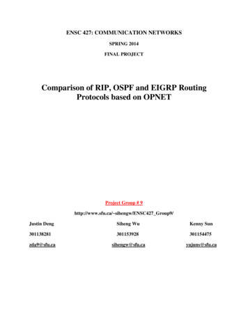
in the MAC layer of the sender plus a propagationdelay. This measurement can be done at the sender sidewithout clock synchronization. Periodically theReceiveFromDelays for each neighbor are averaged tocompute a single node receive delay. If the new nodereceive delay is larger or smaller than the previous nodereceive delay by a certain threshold, then an on demandbeacon will be issued, otherwise there is no beacon.The benefit of choosing an averaged node receivedelay as the metric to denote load of a node is to reducethe channel capture effect [1] at the routing layer. Theneighbor node that captures the channel will be notifiedof a longer delay through the beacon data than itactually experiences. As we can see in section 5.6, thenit will re-route a fraction of packets to other forwardingnodes to reduce the load in this node. By using a singledelay feedback, a node can indicate to all its neighborsto react cooperatively, such that the congestion can bereduced more fairly without starving any neighbornodes.4.4. Stateless Non-deterministic GeographicForwarding (SNGF)Before elaborating on SGNF, we introduce twodefinitions: The Neighbor Set of node i: This is the set of nodesthat are inside the radio range R of node i and alsoat least K distance away from node i. Formally, NSi(K) {node K distance(node , node i ) R }. The Forwarding Candidate Set of node i: A set ofnodes that belong to NSi(K) and are at least Kdistance closer to the destination. Formally, FSi(Destination) {node NSi (K) L – L next K }where L is the distance from node i to thedestination and L next is the distance from the nexthop forwarding candidate to the destination. Thesenodes are inside the cross-hatched shaded area asshown in Figure 1. We can easily obtain FSi(Destination) by scanning the NS set of nodes once.123456DFS132121Figure 1. NS and FS definitionsIt is worth noticing that the membership of theneighbor set only depends on the radio range R anddistance K, but the membership of the forwarding setalso depends on the position of destination nodes.Since SPEED nodes only keep the Neighbor Set(NS), not the routing table, the memory requirement isonly proportional to the number of neighbors, whichcan be ignored compared to the vast size of a sensornetwork.Based on the destination of the packet and thecurrent FS, the Stateless Non-deterministic geographicforwarding (SNGF) part of our protocol routes thepacket according to following rules:1.2.3.4.Packets are forwarded only to the nodes thatbelong to the FSi (Destination). If there is no nodeinside the FSi (Destination), packets are dropped.To reduce the chance of such a drop, we deduce alower bound on node density that can virtuallyeliminate such drops from happening (appendix A).SPEED divides the neighbor nodes inside FSi(Destination) into two groups. One group is thenodes that have SendToDelay less than a certainsingle hop delay D. The others are the nodes thathave SendToDelay longer than a certain single hopdelay D.The forwarding candidate is chosen from the firstgroup, and the neighbor node with highest relaySPEED ( L – L next / SendToDelay ) has ahigher probability to be chosen as the forwardingnode. In our approach, we use a discreteexponential distribution to trade off between loadbalancing and optimal path length.If there are no nodes belonging to the first group, arelay ratio is calculated based on the neighborhoodFeedback Closed Loop, which we will discuss inmore detail later. Whether a packet drop will reallyhappen depends on whether a randomly generatednumber between (0,1) is bigger than the relay ratio.In SPEED a packet is dropped only when nodownstream node can guarantee the single hopdelay and an action must be taken to reduce thecongestion. SPEED also provides back-pressure tothe upper stream node which leads to automaticrerouting as we show in section 5.6.SNGF provides two nice properties to meet ourdesign goals. First, since it only sends packets to a nodethat is K nearer to the destination, it gives an upperbound on the number of hops the packet will travel tothe destination (L/K 1). This, together with a singlehop delay guarantee provided by the NeighborhoodClosed Loop Feedback routine and back-pressurererouting (discussed later), can provide a steady state4

end-to-end delay real-time guarantee for ad hoc sensornetworks. Second, SNGF can balance the traffic andreduce congestion by dispersing the packet into a largerelay area. (An analysis on load balance performance isprovided in appendix B). This load balancing isvaluable in a sensor network where the density of nodesis high and the communication bandwidth is scarce andshared. Also load balancing can balance the powerconsumption inside the sensor network to prevent somenodes from dying faster than others.4.5. Neighborhood Feedback Loop (NFL)The Neighborhood Closed Feedback Loop is thekey component that guarantees the single hop delay.The Neighborhood Closed loop is an effective approachto maintaining system performance at a desired value.This has been shown in [13], where a low, targeted missratio of real-time tasks and a high utilization of thecomputational nodes are simultaneously achieved. Herewe want to maintain a single hop delay below a certainvalue D, a performance goal the system builder desires.Since SNGF give us an upper bound on the numberof hops from the source to the destination, once a singlehop delay D guarantee is provided, formally we canprovide the following end-to-end real-time guarantee inSPEED: In steady state, P{ A packet misses its E2Edeadline} 121111231451678158619 4 61 16781 4551 64 1theoretically zero)controller calculates the relay ratio and feeds that backinto SNGF where a drop or relay action is made. TheRelay ratio controller currently implemented is a simplemultiple inputs single output (MISO) proportionalcontroller that takes the miss ratios of all next-hopneighbors as inputs and proportionally calculates therelay ratio as output to the SNGF.The Relay Ratio controller will be activated onlywhen all nodes inside the forwarding set have aSendToDelay delay larger than the desired single hopdelay D, which means that the neighborhood closedfeedback loop will not be invoked unless there is noway to forward the packet to a non-busy node and adrop is absolutely necessary to guarantee the single hopdelay. As we will see later in the backpressurererouting, such a scheme enforces that re-routing has ahigher priority than dropping. In other words, SPEEDwill not drop a packet as long as there is another paththat can meet the delay requirements.4.6. Back-Pressure ReroutingBack-pressure re-routing is naturally generatedfrom collaboration of neighbor feedback loop (NFL)routines as well as the stateless non-deterministicgeographic forwarding (SNGF) part of SPEED withoutany additional control packets required. To be moreexplicit, we introduce this scheme with an example(Figure 3).123333324567383339 9 9 3 323 3339 9 3 323 9339 9 9 3 323 3339 9 3 32where the E2E deadline is given asD (Distance/K 1).We deem it a miss when a packet arrives at a nodewith a single hop delay longer than D, or if there is aloss due to collision, or a forced-drop. The percentageof such misses for the entire node is called the missratio. The responsibility of the neighborhood closedfeedback loop is to force such a miss ratio to convergeto the set point, namely zero.1234555555567891234561234567894 36 2123456123456789 6-12345678519659212345310BooFigure 3. Back-pressure rerouting case one7897252 69811 Neighborhood TableRelay RatioController7SNGFNeighborNodesFigure 2. Neighborhood Feedback Loop (NFL)As shown in Figure 2, the feedback loop isnaturally established through the neighbor beaconexchange we mention in section 5.2. The Relay RatioSuppose in the lower-right area, some heavy trafficappears, which leads to high delay in nodes 9 and 10.Through beacon exchange node 5 will detect that nodes9 and 10 have a higher delay. Since SNGF will reducethe probability of selecting nodes 9 and 10 asforwarding candidates, it will reduce the congestionaround nodes 9 and 10. Since all neighbors of 9 and 10will react the same as node 5, eventually nodes 9 and 10will adjust their delay below the single hop deadlinethrough Back-pressure re-routing.5

Things are not always as simple as in previouscase. A more severe case could happen when all theforwarding neighbors of node 5 are also congested asshown in figure 4.12333332456738333399 833 323 333399 33 323 333399 33 3275 5 4 Boo1234512345678519592310412Figure 4. Back-pressure rerouting case 2In this case, the neighborhood feedback loop isactivated to assist backpressure re-routing. In node 5 acertain percent of packets will be dropped and whendropped they count as a packet with delay D in terms ofcomputing the delay at this node. The increased averagedelay will be detected by upstream nodes, here node 3,which will react in the same way as above. If,unfortunately, node 3 is in the same situation as node 5,further backpressure will be imposed on node 2. In theextreme case, the whole network is congested and thebackpressure will proceed upstream until it reaches thesource, where the source will quench the traffic.Backpressure rerouting is the first choice used bySPEED to reduce the congestion inside the network. Inthis case no packet need be sacrificed. A drop throughthe feedback-closed loop is only necessary when thesituation is poor and there is no alternative except todrop the packet.4.7. Last Mile ProcessSince SPEED is targeted at sensor networks wherethe ID of nodes is not necessary, we don’t care aboutthe ID’s of individual sensor nodes; instead we onlycare about the location of where the sensor data isgenerated.The Last mile process is so called because onlywhen the packet enters into the destination area willsuch a function be activated. All previous packet relaysare controlled by the SNGF routine as mentionedbefore. The nodes inside the destination area complywith the last mile rules and will not be constrained bythe K distance limitation used in SNGF.The Last mile process provides two novel servicesthat fit the scenario of sensor networks: Area-multicastand Area-anycast. The area here is defined by a center-point (x,y,z) and a radius, which mean it’s a sphere. Ingeneral, more complex area definitions can be madewithout jeopardizing the design of the Last mileprocess.The current implementation of the last mile processis relatively simple. Nodes can differentiate the packettype by the PacketType field mentioned in section 4.1.If it’s an anycast packet, the nodes inside thedestination area will deliver the packet to thetransportation layer without relay. If it’s a multicasttype, the nodes inside the destination area which firstreceive the packet coming from the outside of thedestination area will set a TTL. This allows the packetto survive the diameter of the destination area and bebroadcast to the correct radius. Other nodes inside thedestination area will keep a copy of the packet and rebroadcast it. The nodes that are outside the destinationarea will just ignore it. The last mile process for unicastis nearly the same as multicast, except only the nodewith that global ID will deliver the packet to thetransport layer. If the location directory service isprecise, we can expect the additional flooding overheadfor the unicast packets to be small.5. Experimentation and Evaluation5.1. Simulation EnvironmentWe simulate SPEED on GloMoSim [17], which is ascalable discrete-event simulator developed by UCLA.This software provides high fidelity simulation forwireless communication with detailed propagation,radio and MAC layers simulation. Table 1 describes thedetailed setup for the simulator. The communicationparameters are chosen from UCB’s TinyOSimplementation [4] and its mote specification.Transportation Layer UDPRoutingAODV, DSR, GF, SPEEDNetwork LayerIPMAC Layer802.11Radio LayerRADIO-ACCNOISEPropagation modelTWO-RAYBandwidth200Kb/sPayload size32 ByteTERRAIN(2000m, 2000m)Node number100Node placementUniformRadio Range377mTable 1. Simulation settingsWe discovered that using the CSMA/CA protocolavailable in GloMoSim introduces a high packet lossratio due to the hidden terminal problems that arecommon in congested multi-hop sensor networks,6

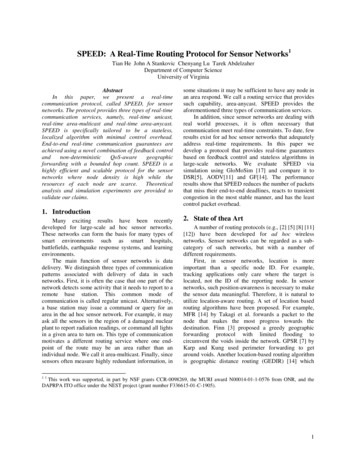
300250E2E Delay (MS)where collisions tend to be heavy. So instead we used802.11 as an alterative MAC layer protocol. Since ourprotocol stack for the physical motes will not useUDP/IP, which has 28 bytes header overhead, to adjustfor these large overheads, compared to the smallpayload size, another change we made was that thebandwidth was chosen to be double the current motecapability.2001501005.2. Congestion Avoidance50020406080100 120time(S)140160180200Figure 5.A. E2E delay profile of DSR300E2E Delay (MS)25020015010050020406080100 120time(S)140160180200Figure 5.B. E2E delay profile of AODV300E2E Delay (MS)25020015010050020406080100 120time(S)140160180200Figure 5.C. E2E delay profile of GF300250E2E Delay (MS)In a sensor network, where node density is highand bandwidth is scarce, traffic hot spots can be easilycreated. In turn, such hot spots may interfere with realtime guarantees of critical traffic in the network. Toalleviate this problem, SPEED supports a combinationof QoS-aware routing and back-pressure congestioncontrol suitable for sensor networks.To test the aforementioned capabilities, we used across traffic scenario, where 4 nodes at the upper leftcorner of the terrain send periodic data to a base stationat the lower right corner and 4 nodes at the lower leftcorner send periodic data to the base station at the upperright corner. The average hop count between the nodeand base station is about 10 hops. Each node generates1 CBR flow with a rate of 0.5 packet/second. To createcongestion, at time 40 seconds, one heavy flow iscreated between two randomly chosen nodes in themiddle of the terrain with a rate of 50 packets/second.This flow disappears at time 120 seconds into the run.This heavy flow introduces a step change into thesystem, which is an abrupt change that stress-testsSPEED adaptation capabilities to reveal its transientstate response.We repeated the experiments with the same trafficload settings but different routing algorithms tocompare SPEED to DSR, AODV, and GF. For eachrouting algorithm we report the average performance of16 runs with different random seeds. Figures 5.A, 5.B5.C and 5.D plot the end-to-end (E2E) delay profiles forthe four different routing algorithms. At each point intime, we average the E2E delays of all the packets fromthe 128 flows (16 runs with 8 flows each). Forlegibility, any average E2E delay larger than 300milliseconds is drawn as 300 milliseconds in thefigures. Separately, Figure 6 uses statisticalcomparative boxplots to show the number of packetslost during the congestion. In these boxplots, the line inthe middle of the box denotes the median value of thedata set. The bottom and top of the box are the 25th and75th percentiles. T-shaped lines here denote themaximum and minimum value of the data set.20015010050020406080100 120time(S)140160180200Figure 5.D E2E delay profile of SPEED7

100#Packets Lost806040200DSRAODVGFSPEEDFigure 6. Number of packets lost during congestionWhen DSR and AODV begin, they need toperform route acquisition to discover a path to thedestination, causing a large delay (Figures 5.A and 5.B)for the first packet (10 20 times longer than the delayof the following packets). On the other hand GF andSPEED don’t suffer from this feature. In theseprotocols, the first packet has same delay as thefollowing packets. Without an initial delay cost, GF andSPEED are more suitable for real-time applications likeacoustic tracking where the base station sends theactuation commands to the sensor group, which isdynamically changing as the target moves. In such ascenario, DSR and AODV need to perform routeacquisition repeatedly in order to track the target.In general, both GF and SPEED tend to forwardthe packet at each step as close to the destination aspossible, which leads to less overall E2E delay than forDSR and AODV (See Figures 5.C and 5.D)At time 40 sec when the heavy flow appears, thesystem enters

TTL: Time To Live field is the hop limit used for last mile processing. Payload. 4.2. Neighbor Beacon Exchange SPEED relies on neighborhood information to compute per-hop delays. Periodically and asynchronously, every node broadcasts a beacon packet to its neighbors. Each beacon packet has three fields: (ID, Position, node receive delay)