Transcription
The Vectorial Lambda-CalculusPablo Arrighia,b , Alejandro Dı́az-Caroc,e , Benoı̂t Valirond,ea ENS-Lyon,Laboratoire LIP, Francede Grenoble, Laboratoire LIG, Francec Université Paris-Ouest Nanterre La Défense, Franced University of Pennsylvania, CIS Department, USAe INRIA Paris-Rocquencourt, Franceb UniversitéAbstractWe describe a type system for the linear-algebraic lambda-calculus. The type systemaccounts for the linear-algebraic aspects of this extension of lambda-calculus: it is ableto statically describe the linear combinations of terms that will be obtained when reducingthe programs. This gives rise to an original type theory where types, in the same way asterms, can be superposed into linear combinations. We prove that the resulting typedlambda-calculus is strongly normalising and features a weak subject reduction. Finally,we show how to naturally encode matrices and vectors in this typed calculus.1. Introduction1.1. (Linear-)algebraic lambda-calculiA number of recent works seek to endow the λ-calculus with a vector space structure.This agenda has emerged simultaneously in two different contexts. The field of Linear Logic considers a logic of resources where the propositionsthemselves stand for those resources – and hence cannot be discarded nor copied.When seeking to find models of this logic, one obtains a particular family of vectorspaces and differentiable functions over these. It is by trying to capture back thesemathematical structures into a programming language that Ehrhard and Regnierhave defined the differential λ-calculus [21], which has an intriguing differentialoperator as a built-in primitive and an algebraic module of the λ-calculus termsover natural numbers. Vaux [34] has focused his attention on a ‘differential λcalculus without differential operator’, extending the algebraic module to positivereal numbers. He obtained a confluence result in this case, which stands even in theuntyped setting. More recent works on this algebraic λ-calculus tend to considerarbitrary scalars [31, 20, 1].Email addresses: pablo.arrighi@imag.fr (Pablo Arrighi), alejandro@diaz-caro.info (AlejandroDı́az-Caro), benoit.valiron@monoidal.net (Benoı̂t Valiron)Preprint submitted to arXivAugust 5, 2013
The field of Quantum Computation postulates that, as computers are physicalsystems, they may behave according to the quantum theory. It proves that, if thisis the case, novel, more efficient algorithms are possible [30, 23] – which have noclassical counterpart. Whilst partly unexplained, it is nevertheless clear that thealgorithmic speed-up arises by tapping into the parallelism granted to us ‘for free’by the superposition principle; which states that if t and u are possible states ofa system, then so is the formal linear combination of them α · t β · u (with αand β some arbitrary complex numbers, up to a normalizing factor). The ideaof a module of λ-terms over an arbitrary scalar field arises quite naturally in thiscontext. This was the motivation behind the linear-algebraic λ-calculus, or Linealfor short, by Dowek and one of the authors [6], who obtained a confluence resultwhich holds for arbitrary scalars and again covers the untyped setting.These two languages are rather similar: they both merge higher-order computation, beit terminating or not, in its simplest and most general form (namely the untyped λcalculus) together with linear algebra in its simplest and most general form also (theaxioms of vector spaces). In fact they can simulate each other [17]. Our starting point isthe second one, Lineal, because its confluence proof allows arbitrary scalars and becauseone has to make a choice. Whether the models developed for the first language, and thetype systems developed for the second language, carry through to one another via theirreciprocal simulations, is a topic of future investigation.1.2. Other motivations to study (linear-)algebraic lambda-calculiThe two languages are also reminiscent of other works in the literature: Algebraic and symbolic computation. The functional style of programming is basedon the λ-calculus together with a number of extensions, so as to make everydayprogramming more accessible. Hence since the birth of functional programmingthere have been several theoretical studies on extensions of the λ-calculus in orderto account for basic algebra (see for instance Dougherty’s algebraic extension [19] fornormalising terms of the λ-calculus) and other basic programming constructs suchas pattern-matching [12, 3], together with sometimes non-trivial associated typetheories [29]. Whilst this was not the original motivation behind (linear-)algebraicλ-calculi, they could still be viewed as an extension of the λ-calculus in order tohandle operations over vector spaces and make programmingmore accessible uponthem. The main difference in approach is that the λ-calculus is not seen here as acontrol structure which sits on top of the vector space data structure, controllingwhich operations to apply and when. Rather, the λ-calculus terms themselves canbe summed and weighted, hence they actually are vectors, upon which they canalso act. Parallel and probabilistic computation. The above intertwinings of concepts areessential if seeking to represent parallel or probabilistic computation as it is thecomputation itself which must be endowed with a vector space structure. Theability to superpose λ-calculus terms in that sense takes us back to Boudol’s parallelλ-calculus [8] or de Liguoro and Piperno’s work on non-deterministic extensions ofλ-calculus [13], as well as more recent works such as [28, 10, 16]. It may also2
be viewed as being part of a series of works on probabilistic extensions of calculi,e.g. [9, 24] and [14, 27, 15] for λ-calculus more specifically.Hence (linear-)algebraic λ-calculi can be seen as a platform for various applications,ranging from algebraic computation, probabilistic computation, quantum computationand resource-aware computation.1.3. The languageThe language we consider in this paper will be called the vectorial lambda-calculus,denoted by λvec . It is derived from Lineal [6]. This language admits the regular constructsof lambda-calculus: variables x, y, . . ., lambda-abstractions λx.s and application (s) t.But it also admits linear combinations of terms: 0, s t and α · s are terms, where thescalar α ranges over a ring. As in [6], it behaves in a call-by-value oriented manner, in thesense that (λx.r) (s t) first reduces to (λx.r) s (λx.r) t until basis terms (i.e. values)are reached, at which point beta-reduction applies.The set of the normal forms of the terms can then be interpreted as a module and theterm (λx.r) s can be seen as the application of the linear operator (λx.r) to the vector s.The goal of this paper is to give a formal account of linear operators and vectors at thelevel of the type system.1.4. Our contributions: The typesOur goal is to characterize the vectoriality of the system of terms, as summarized bythe slogan:If s : T and t : R then α · s β · t : α · T β · R.In the end we achieve a type system such that: The typed language features a slightly weakened subject reduction (cf. Theorem 4.1). The typed language features strong normalization (cf. Theorem 5.13).PP In general, if t has type i αi ·Ui , then it must reduce to aPt0 of the form ij βij ·bij ,where: the bij ’s are basis terms of unit type Ui , and ij βij αi . (cf. Theorem 6.1). In particular finite vectors and matrices and tensorial products can be encodedwithin λvec . In this case, the type of the encoded expressions coincides with theresult of the expression (cf. Theorem 6.2).Beyond these formal results, this work constitutes a first attempt to describe a naturaltype system with type constructs α· and and to study their behaviour.3
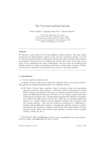
1.5. Directly related worksThis paper is part of a research path [33, 2, 6, 32, 11, 4, 18] to design a typedlanguage where terms are quantified (they can be interpreted as probability distributionsor quantum superpositions of data and programs) and the types are quantified (theyprovide the propositions for a probabilistic or quantum logic via Curry-Howard).Along this path, a first step was accomplished in [4] with scalars in the type system.If α is a scalar and Γ t : T is a valid sequent, then Γ α · t : α · T is a valid sequent.When the scalars are taken to be positive real numbers, the developed language actuallyprovides a static analysis tool for probabilistic computation. However, it fails to addressthe following issue: without sums but with negative numbers, the term representing“true false”, namely λx.λy.x λx.λy.y, is typed with 0 · (X (X X)), a typewhich fails to exhibit the fact that we have a superposition of terms.A second step was accomplished in [18] with sums in the type system. In this case,if Γ s : S and Γ t : T are two valid sequents, then Γ s t : S T is a validsequent. However, the language considered is only the additive fragment of Lineal, itleaves scalars out of the picture. For instance, λx.λy.x λx.λy.y, does not have a type,due to its minus sign. Each of these two contributions required renewed, careful andlengthy proofs about their type systems, introducing new techniques.The type system we propose in this paper builds upon these two approaches: itincludes both scalars and sums of types, thereby reflecting the vectorial structure ofthe terms at the level of types. Interestingly, combining the two separate features of[4, 18] raises subtle novel issues, which we identify and discuss. Equipped with those twovectorial type constructs, the type system is indeed able to capture some fine-grainedinformation about the vectorial structure of the terms. Intuitively, this means keepingtrack of both the ‘direction’ and the ‘amplitude’ of the terms.A preliminary version of this paper has appeared in [5].1.6. Plan of the paperIn Section 2, we present the language. We discuss the differences with the originallanguage Lineal [6]. In Section 3, we explain the problems arising from the possibility ofhaving linear combinations of types, and elaborate a type system that addresses thoseproblems. Section 4 is devoted to subject reduction. We first say why the standardformulation of subject reduction does not hold. Second we state a slightly weakenednotion of the subject reduction theorem, and we prove this result. In Section 5, we provestrong normalisation. Finally we close the paper in Section 6 with theorems about theinformation brought by the type judgements, both in the general and the finitary cases(matrices and vectors).2. The termsWe consider the untyped language λvec described in Figure 1. It is based on Lineal[6]: terms come in two flavours, basis terms which are the only ones that will substitutea variable in a β-reduction step, and general terms. We use Krivine’s notation [26] forfunction application: The term (s) t passes the argument t to the function s.In addition to β-reduction, there are fifteen rules stemming from the oriented axiomsof vector spaces [6], specifying the behaviour of sums and products. We divide the rules4
Terms:Basis terms:Group E:0·t 01·t tα·0 0α · (β · t) (α β) · tα · (t r) α · t α · rr, s, t, u :: b (t) rb :: x λx.tGroup F:α · t β · t (α β) · tα · t t (α 1) · tt t (1 1) · tt 0 tGroup B:(λx.t) b t[b/x] 0 α·t t rGroup A:(t r) u (t) u (r) u(t) (r u) (t) r (t) u(α · t) r α · (t) r(t) (α · r) α · (t) r(0) t 0(t) 0 0t rt rt rt rt rα·t α·ru t u r(u) t (u) r(t) u (r) uλx.t λx.rFigure 1: Syntax, reduction rules and context rules of λvec .in groups: Elementary (E), Factorisation (F), Application (A) and the Beta reduction(B). A general term t is thought of as a linear combination of terms α ·r β ·r0 . When weapply s to this superposition, (s) t reduces to α · (s) r β · (s) r0 . Terms are consideredmodulo associativity and commutativity of the operator , making the reduction into anAC-rewrite system [25]. Scalars (notation α, β, γ, . . . ) form a ring (S, , ). The typicalring we consider in the examples is the ring of complex numbers. In particular, we shalluse the shortcut notation s t in place of s ( 1) · t.The set of free variables of a term is defined as usual: the only operator bindingvariables is the λ-abstraction. The operation of substitution on terms (notation t[b/x])is defined in the usual way for the regular lambda-term constructs, by taking care ofvariable renaming to avoid capture. For a linear combination, the substitution is definedas follows: (α · t β · r)[b/x] α · t[b/x] β · r[b/x].Note that we need to choose a reduction strategy. For example, the term (λx.(x) x)(y z) cannot reduce to both (λx.(x) x) y (λx.(x) x) z and (y z) (y z). Indeed, theformer normalizes to (y) y (z) z whereas the latter normalizes to (y) z (y) y (z) y (z) z;which would break confluence. As in [6, 4, 18], we consider a call-by-value reductionstrategy: The argument of the application is required to be a base term, cf. Group B.2.1. Relation to LinealAlthough strongly inspired from Lineal, the language λvec is closer to [17, 4, 18].Indeed, Lineal considers some restrictions on the reduction rules, for example α · t β ·t (α β) · t is only allowed when t is a closed normal term. These restrictions areenforced to ensure confluence in the untyped setting. Consider the following example.Let Yb (λx.(b (x) x)) λx.(b (x) x). Then Yb reduces to b Yb . So the termYb Yb reduces to 0, but also reduces to b Yb Yb and hence to b, breakingconfluence. The above restriction forbids the first reduction, bringing back confluence.In our setting we do not need it because Yb is not well-typed. If one considers a typedlanguage enforcing strong normalisation, one can wave many of the restrictions andconsider a more canonical set of rewrite rules [17, 4, 18]. Working with a type systemenforcing strong normalisation (as shown in Section 5), we follow this approach.5
2.2. Booleans in the vectorial lambda-calculusWe claimed in the introduction that the design of Lineal was motivated by quantumcomputing; in this section we develop this analogy.Both in λvec and in quantum computation one can interpret the notion of booleans.In the former we can consider the usual booleans λx.λy.x and λx.λy.y whereas in thelatter we consider the regular quantum bits true 0i and false 1i.In λvec , a representation of if r then s else t needs to take into account the specialrelation between sums and applications. We cannot directly encode this test as the usual((r) s) t. Indeed, if r, s and t were respectively the terms true, s1 s2 and t1 t2 , the term((r) s) t would reduce to ((true) s1 ) t1 ((true) s1 ) t2 ((true) s2 ) t1 ((true) s2 ) t2 ,then to 2 · s1 2 · s2 instead of s1 s2 . We need to “freeze” the computations in eachbranch of the test so that the sum does not distribute over the application. For thatpurpose we use the well-known notion of thunks [6]: we encode the test as {((r) [s]) [t]},where [ ] is the term λf. with f a fresh, unused term variable and where { } is theterm ( )λx.x. The former “freezes” the linearity while the latter “releases” it. Then theterm if true then (s1 s2 ) else (t1 t2 ) reduces to the term s1 s2 as one could expect.Note that this test is linear, in the sense that the term if (α·true β ·false) then s else treduces to α · s β · t.This is similar to the quantum test that can be found e.g. in [33, 2]. Quantumcomputation deals with complex, linear combinations of terms, and a typical computationis run by applying linear unitary operations on the terms, called gates. For example, theHadamardgate H acts on the space of booleans spanned by true and false. It sends true to 22 (true false) and false to 22 (true false). If x is a quantum bit, the value(H) x can be represented as the quantum test 22(H) x : if x then(true false) else(true false).22As developed in [6], one can simulate this operation in λvec using the test constructionwe just described:(" #! " #) 2222{(H) x} : (x)· true · false· true · false.2222 Note that the thunks are necessary: without thunks the term ((x) ( 22 · true 22 · false)) ( 22 ·true 22 ·false) would reduce to the term 12 (((x) true) true ((x) true) false ((x) false) true ((x) false) false), which is fundamentally different from the term Hwe are trying to emulate.With this procedure we can “encode” any matrix. If the space is of some generaldimension n, instead of the basis elements true and false we can choose for i 1 ton the terms λx1 . · · · .λxn .xi ’s to encode the basis of the space. We can also take tensorproducts of qubits. We come back to this encodings in Section 6.3. The type systemThis section presents the core definition of the paper: the vectorial type system.6
3.1. IntuitionsBefore diving into the technicalities of the definition, we discuss the rational behindthe construction of the type-system.3.1.1. Superposition of typesWe want to incorporate the notion of scalars in the type system. If A is a valid type,the construction α · A is also a valid type and if the terms s and t are of type A, the termα · s β · t is of type (α β) · A. This was achieved in [4] and it allows us to distinguishbetween the functions λx.(1 · x) and λx.(2 · x): the former is of type A A whereas thelatter is of type A (2 · A).The terms true and false can be typed in the usual way with B X (X X), fora fixed type X. So let us consider the term 22 · (true false). Using the above additionto the type system, this term should be of type 0 · B, a type which fails to exhibit thefact that we have a superposition of terms. For instance, applying the Hadamard gateto this term produces the term false of type B: the norm would then jump from 0 to 1.This time, the problem comes from the fact that the type system does not keep track ofthe “direction” of a term.To address this problem we must allow sums of types. For instance,provided that T X (Y X) and F X (Y Y ), we can type the term 22 · (true false) with 22 · (T F), which has L2 -norm 1, just like the type of false has norm one. At this stage the type system is able to type the term H λx.{((x) [ 22 · true 22 · false]) [ 22 · true 22 · false]}, with ((I 22 .(T F)) (I 22 .(T F)) I T ) T with I an identity type of the form Z Z and T any fixed type. Let us now try to type the term (H) true. This is possible by taking T to be 22 ·(T F). But then, if we want to type the term (H) false, T needs to be equal to 22 · (T F).It follows that we cannot type the term (H) ( 22 · true 22 · false) since there is nopossibility to conciliate the two constraints on T .To address this problem, we need a forall construction in the type system, makingit à la System F. The term H can now be typed with T.((I 22 · (T F)) (I 22 · (T F)) I T ) T and the types T and F are updated to be respectively XY.X (Y X) and XY.X (Y Y ). The terms (H) true and (H) false can 2both be well-typed with respective types 2 · (T F) and 22 · (T F), as expected.3.1.2. Type variables, units and general typesBecause of the call-by-value strategy, variables must range over types that are notlinear combination of other types, i.e. unit types. To illustrate this necessity, considerthe following example. Suppose we allow variables to have scaled types, such as α · U .Then the term λx.x y could have type (α · U ) α · U V (with y of type V ). Let bbe of type U , then (λx.x y) (α · b) has type α · U V , but then(λx.x y) (α · b) α · (λx.x y) b α · (b y) α · b α · y ,which is problematic since the type α·U V does not reflect such a superposition. Hence,the left side of an arrow will be required to be a unit type.7
Type variables, however, do not always have to be unit type. Indeed, a forall of ageneral type was needed in the previous section in order to type the term H. But weneed to distinguish a general type variable from a unit type variable, in order to makesure that only unit types appear at the left of arrows. Therefore, we define two sorts oftype variables: the variables X to be replaced with unit types, and X to be replaced withany type (we use just X when we mean either one). The type X is a unit type whereasthe type X is not.In particular, the type T is now XY.X Y X, the type F is XY.X Y Yand the type of H is!!! 22· (T F) I · (T F) I X X. X.I 22Notice how the left sides of all arrows remain unit types.3.1.3. The term 0The term 0 will naturally have the type 0 · T , for any inhabited type T . We could alsoconsider to add the equivalence R 0 · T R as in [4]. However, consider the followingexample. Let λx.x be of type U U and let t be of type T . The term λx.x t t isof type (U U ) 0 · T , that is, (U U ). Now choose b of type U : we are allowedto say that (λx.x t t) b is of type U . This term reduces to b (t) b (t) b. But ifthe type system is reasonable enough, we should at least be able to type (t) b. However,since there is no constraints on the type T , this is difficult to enforce.The problem comes from the fact that along the typing of t t, the type of t is lostin the equivalence (U U ) 0 · T U U . The only solution is to not discard 0 · T ,that is, to not equate R 0 · T and R.3.2. FormalisationWe now give a formal account of the type system: we first describe the language oftypes, then present the typing rules.3.2.1. Definition of typesTypes are defined in Figure 2 (top). They come in two flavours: unit types and generaltypes, that is, linear combinations of types. Unit types include all types of System F [22,Ch. 11] and intuitively they are used to type basis terms. The arrow type admits only aunit type in its domain. This is due to the fact that the argument of a lambda-abstractioncan only be substituted by a basis term, as discussed in Section 3.1.2. The type systemfeatures two sorts of variables: unit variables X and general variables X. The former canonly be substituted by a unit type whereas the latter can be substituted by any type. Weuse the notation X when the type variable is unrestricted. The substitution of X by U(resp. X by S) in T is defined as usual and is written T [U/X] (resp. T [S/X]). We usethe notation T [A/X] to say: “if X is a unit variable, then A is a unit type and otherwiseA is a general type”. In particular, for a linear combination, the substitution is definedas follows: (α · T β · R)[A/X] α · T [A/X] β · R[A/X]. We also use the vectorial X] for T [A1 /X1 ] · · · [An /Xn ] if X X1 , . . . , Xn and A A1 , . . . , An , andnotation T [A/ also X for X1 . . . Xn X1 . . . . . Xn .8
T, R, S :: U α · T T R XU, V, W :: X U T X.U X.UTypes:Unit types:1·T Tα · (β · T ) (α β) · Tα · T α · R α · (T R)Γ t:TaxΓ, x : U x : Uα · T β · T (α β) · TT R R TT (R S) (T R) SΓ 0:0·TΓ t:nX αi · X.(U Ti )Γ, x : U t : T0IΓ λx.t : U TΓ r:mX j /X] βj · U [Aj 1i 1Γ (t) r :mn XX I E j /X] αi βj · Ti [Ai 1 j 1Γ t:nXαi · UiX / F V (Γ)i 1Γ t:nXΓ t: IΓ t:αi · X.Uii 1Γ t:TΓ α·t:α·Tαi · X.Uii 1nX Eαi · Ui [A/X]i 1Γ t:TαInXΓ r:RΓ t r:T R IΓ t:TT RΓ t:R Figure 2: Types and typing rules of λvec . We use X when we do not want to specify if it is X or X, thatis, unit variables or general variables respectively. In T [A/X], if X X, then A is a unit type, and ifX X, then A can be any type. We also may write I and I (resp. E and E ) when we need to specifywhich kind of variable is being used.9
The equivalence relation on types is defined as a congruence. Notice that thisequivalence makes the types into a weak module over the scalars: they almost form amodule save from the fact that there is no neutral element for the addition. The type0 · T is not the neutral element ofPthe addition.We may use the summation ( ) notation without ambiguity, due to the associativityand commutativity equivalences of .3.2.2. Typing rulesThe typing rules are given also in Figure 2 (bottom). Contexts are denoted by Γ, , etc. and are defined as sets {x : U, . . . }, where x is a term variable appearing onlyonce in the set, and U is a unit type. The axiom (ax) and the arrow introductionrule ( I ) are the usual ones. The rule (0I ) to type the term 0 takes into accountthe discussion in Section 3.1.3. This rule also ensures that the type of 0 is inhabited,discarding problematic types like 0 · X.X. Any sum of typed terms can be typedusing Rule ( I ). Similarly, any scaled typed term can be typed with (αI ). Rule ( )ensures that equivalent types can be used to type the same terms. Finally, the particularform of the arrow-elimination rule ( E ) is due to the rewrite rules in group A thatdistribute sums and scalars over application. The need and use of this complicatedarrow elimination can be illustrated by the following three examples.Example 3.1. Rule ( E ) is easier to read for trivial linear combinations. It statesthat provided that Γ s : X.U S and Γ t : V , if there exists some type Wsuch that V U [W/X], then since the sequent Γ s : V S[W/X] is valid, we alsohave Γ (s) t : S[W/X]. Hence, the arrow elimination here does an arrow and a forallelimination at the same time.Example 3.2. Consider the terms b1 and b2 , of respective types U1 and U2 . The termb1 b2 is of type U1 U2 . We would reasonably expect the term (λx.x) (b1 b2 ) to bealso of type U1 U2 . This is the case thanks to Rule ( E ). Indeed, type the term λx.xwith the type X.X X and we can now apply the rule. Notice that we could not typesuch a term unless we eliminate the forall together with the arrow.Example 3.3. A slightly more evolved example is the projection of a pair of elements.It is possible to encode in System F the notion of pairs and projections: hb, ci λx.((x) b) c, hb0 , c0 i λx.((x) b0 ) c0 , π1 λx.(x) (λy.λz.y) and π2 λx.(x) (λy.λz.z).Provided that b, b0 , c and c0 have respective types U , U 0 , V and V 0 , the type of hb, ciis X.(U V X) X and the type of hb0 , c0 i is X.(U 0 V 0 X) X. Theterm π1 and π2 can be typed respectively with XY Z.((X Y X) Z) Z and XY Z.((X Y Y ) Z) Z. The term (π1 π2 ) (hb, ci hb0 , c0 i) is then typableof type U U 0 V V 0 , thanks to Rule ( E ). Note that this is consistent with therewrite system, since it reduces to b c b0 c0 .3.3. Example: Typing HadamardIn this Section, we formally show how to retrieve the type that was discussed inSection 3.1.2, for the term H encoding the Hadamard gate.Let true λx.λy.x and false λx.λy.y. It is easy to check that true : XY.X Y X,10
false : XY.X Y Y.We also define the following superpositions:1 i · (true false)21 i · (true false).2andIn the same way, we define1 · (( XY.X Y X) ( XY.X Y Y)),21 · (( XY.X Y X) ( XY.X Y Y)).2Finally, we define [t] λx.t, where x / F V (t) and {t} (t) I. So {[t]} t. Thenit is easy to check that [ i] : I and [ i] : I . In order to simplify thenotation, let F (I ) (I ) (I X). Thenx:F x:Faxx : F [ i] : I x : F (x) [ i] : (I ) (I X) Ex : F [ i] : I x : F (x) [ i][ i] : I Xx : F {(x) [ i][ i]} : X λx.{(x) [ i][ i]} : F X λx.{(x) [ i][ i]} : X.((I ) (I E E I) (I X)) X INow we can apply Hadamard to a qubit and get the right type. Let H be the termλx.{(x) [ i][ i]} true : X. Y.X Y X H : X.((I ) (I H : ((I ) (I ) (I X)) X) (I )) E true : Y.(I ) Y (I ) true : (I ) (I (H) true : E) (I ) E E4. Subject reductionAs we will now explain, the usual formulation of subject reduction is not directlysatisfied. We discuss the alternatives and opt for a weakened version of subject reduction.4.1. Principal types and subtyping alternativesSince the terms of λvec are not explicitly typed, we are bound to have sequents suchas Γ t : T1 and Γ t : T2 with distinct types T1 and T2 for the same term t. UsingRules ( I ) and (αI ) we get the valid typing judgement Γ α · t β · t : α · T1 β · T2 .Given that α · t β · t reduces to (α β) · t, a regular subject reduction would ask forthe valid sequent Γ (α β) · t : α · T1 β · T2 . But since in general we do not haveα · T1 β · T2 (α β) · T1 (α β) · T2 , we need to find a way around this.11
A first approach would be to use the notion of principal types. However, since ourtype system includes System F, the usual examples for the absence of principal typesapply to our settings: we cannot rely upon this method.A second approach would be to ask for the sequent Γ (α β) · t : α · T1 β · T2to be valid. If we force this typing rule into the system, it seems to solve the issue butthen the type of a term becomes pretty much arbitrary: with typing context Γ, the term(α β) · t would then be typed with any combination γ · T1 δ · T2 , where α β γ δ.The approach we favour in this paper is via a notion of order on types. The order,denoted with v, will be chosen so that the factorisation rules make the types of termssmaller. We will ask in particular that (α β) · T1 v α · T1 β · T2 and (α β) · T2 vα · T1 β · T2 whenever T1 and T2 are types for the same term. This approach can alsobe extended to solve a second pitfall coming from the rule t 0 t. Indeed, althoughx : X x 0 : X 0 · T is well-typed for any inhabited T , the sequent x : X x : X 0 · Tis not valid in general. We therefore extend the ordering to also have X v X 0 · T .Notice that we are not introducing a subtyping relation with this ordering. Forexample, although (α β) · λx.λy.x : (α β) · X.X (X X) is valid and (α β) · X.X (X X) w α · X.X (X X) β · XY.X (Y Y), the sequent (α β) · λx.λy.x : α · X.X (X X)
The language we consider in this paper will be called the vectorial lambda-calculus, denoted by vec. It is derived from Lineal [6]. This language admits the regular constructs of lambda-calculus: variables x;y;:::, lambda-abstractions x:s and application (s)t. But it also admits linear combinations of terms: 0, s t and s are terms, where the