Transcription
Lambda Calculus - Step by StepHelmut Brandl(firstname dot lastname at gmx dot net)AbstractThis little text gives a step by step introduction into untypedlambda calculus. All needed theory is explained and no special knowhow is assumed. Although elementary, all important theorems aboutuntyped lambda calculus including some undecidability theorems aregiven and proved within this text.It has been tried to use a notation which is easy to understandwith a lot of graphic notation to support a good intuition about thepresented material.Contents1 Motivation32 Inductive Sets and Relations2.1 Inductive Sets . . . . . . . . . . . . . . . . . . . . . . .2.2 Inductive Relations . . . . . . . . . . . . . . . . . . . .2.3 Diamonds and Confluence . . . . . . . . . . . . . . . .557123 Lambda Terms3.1 Basic Definitions . . . . . . . . . . . . . . . . . . . . .3.2 Simple Computation with Combinators . . . . . . . .3.3 Confluence - Church Rosser Theorem . . . . . . . . . .171722254 Computable Functions4.1 Boolean Functions . . . . . . . .4.2 Composition of Decomposition of4.3 Numeric Functions . . . . . . . .4.4 Primitive Recursion . . . . . . .32323334361. . . .Pairs . . . . . . .
4.54.6Some Primitive Recursive Functions . . . . . . . . . .General Recursion . . . . . . . . . . . . . . . . . . . .5 Undecidability3741432
1MotivationWhy study lambda calculus?Let us put the question in some historical context. At the beginning of the 20th century the famous mathematician David Hilbertchallenged the mathematical community by the statement that mathematical problems must be decidable. At the 1930 annual meeting ofthe Society of German Scientists and Physicians he made his famousquote “We must know, we will know”.“Entscheidungsproblem” (DecisionProblem). Mathematics must beChallenge decidable. “We must know, we willknow!”David HilbertKurt Gödel (1931):Alonzo Church (1936):Alan Turing (1936):Incompleteness TheoremsLambda CalculusTuring MachineThe young mathematician Kurt Gödel attended the meeting andexpressed some doubts to his collegues about the general decidabilityof mathematical statements. One year later in 1931 he published hisfamous incompleteness theorems [3]. He proved that for all consistent formal systems which are capable of expressing logic and doingsimple arithmetics there are certain statements which are not provable withing the system but true. These incompleteness theorems areconsidered as the first serious blow of Hilbert’s program.Five years later Alonzo Church [2] and Alan Turing [1] independently proved that the decision problem cannot be solved. Alonzo3
Church invented the lambda calculus and Alan Turing his automaticmachine (today called Turing machine) which are both equivalent inexpressiveness.Although Church’s lambda calculus has been published slightly before Alan Turing published his paper on automatic machines usuallyTuring machines are used define computability and decidability. Turing machines resemble more the structure of modern computers thanlambda calculus. A programming language is called Turing completeif all possible algorithms can be coded within the language. Nobodytalks about lambda complete.However lambda calculus is a quite fascinating model of computation. The lambda calculus invented by Alonzo Church is remarkablysimple. It consists just of variables, function applications and lambdaabstractions. But the calculus is sufficiently powerful to express allcomputable functions and decision procedures.Beside its expressive power lambda calculus is used as the theoretical base of functional languages like Haskell, ML, F#.In this paper we explain the lambda calculus in its purest form asuntyped lambda calculus.4
22.1Inductive Sets and RelationsInductive SetsSet Notation A set is an unordered collection of objects. If theobject a is an element of the set A we write a A.A set A is a subset of set B if all elements of the set A are alsoelements of the set B. The symbol is used to express the subsetrelation. The operator : is used to express that something is validby definition. Therefore the subset relation is defined symbolically byA B : a . a A a B. The statement A B can always bereplaced by its definition a . a A a B and vice versa.The double arrow is used to express implication. p q statesthe assertion that having a proof of p we can conclude q. The assertionp q is proved by assuming p and deriving the validity of q.Rule Notation We have often several premises which are neededreach a conclusion. E.g. we might have the assertion p1 p2 . . . c.p1p2p ,p ,.Then we use the rule notation 1 2or . to express the samec.cfact. Evidently the order of the premises is not important.Variable in rules are universally quantified. Therefore we can statethe subset definition a . a A a B. in rule notation morea Acompactly and better readable as. It should be clear froma Bthe context which symbols denote variables.Inductive Definition of Sets Rules can be used to define setsinductively. The set of even numbers E can be defined by the twon Erules 0 E and. A set defined by rules is the least setn 2 Ewhich satisfies the rules. The set E of even number must contain thenumber 0 and with all numbers n it contains also the number n 2.The fact that some object is an element of an inductively definedset must be established by an arbitrarily long but finite sequence ofapplications of the rules which define the set. A proof of 4 Econsists of a proof of 0 E by application of the first rule and thentwo applications of the second rule to reach 2 E and 4 E.5
Rule Induction If we have the fact that an object is an elementof some inductively defined set then we can be sure that it is in theset because of one of the rules which define the set.This can be used to prove facts by rule induction. Suppose we wantto prove that some property p is shared by all even numbers. We cann Eexpress this statement by the rule. Note that variables inp(n)rules are implicitly universally quantified, i.e. the rule expresses thestatement n . n E p(n).It is possible to prove this statement by induction on n E. Sucha proof consists of a proof of the statement for each rule. In the caseof even numbers there are two rules.For the first rule we have to prove the the number 0 satisfies theproperty p(0).For the second rule we assume that n E because there is someother number m already in the set of even numbers E and n m 2.I.e. we have to prove the goal p(m 2) under the premise m E.Because of the premise m E we can assume the induction hypothesisp(m). I.e. we can assume m E and p(m) and derive the validity ofp(m 2).If the proof succeeds for both rules we are allowed to conclude thatthe property p is satisfied by all even numbers.Natural Number Induction It is not difficult to see that theusual law of induction on natural numbers is just a special case of ruleinduction. We can define the set of natural numbers inductively N bythe rules1. 0 Nn N2.n0 Nwhere n0 denotes the successor of n i.e. 3 is just a shorthand for 0000 .The usual induction law of natural numbers allows to prove aproperty p for all natural number by a proof of p(0) and a proofof n . p(n) p(n0 ) which are exactly the requirements of a proof byrule induction.Grammar Notation In some cases it is convenient to define a setby a grammar. E.g. we can define the set of natural numbers by all6
terms n generated by the grammarn :: 0 n0i.e. we can use the corresponding induction law to prove that all termsgenerated by the grammar satisfy a certain property.This definition is just a special form of the definition of the set ofnatural numbers N by the rules1. 0 Nn N2.n0 N2.2Inductive RelationsRelations n-ary relations are just sets of n-tuples. A binary relation r over the sets A and B is a subset of the cartesian productr A B.We use the notations (a, b) r, r(a, b) and a r b to denote the factthat the pair (a, b) with a A and b B figure in the relation r.In this paper we need only endorelations i.e. binary relations wherethe domain A and the range B of the relation are the same set.Relation Closure As with sets, relations can be defined inductively.Definition 2.1. The transitive closure r of a relation r is definedby the rules1.r(a, b)r (a, b)2.r (a, b), r(b, c)r (a, c)The rules can be displayed graphically. The premises are markedblue and the conclusion is marked red.r r arabr brcr We calledthe transitive closure of r, but the fact that r istransitive needs a proof.7
Theorem 2.2. The transitive closure r of the relation r is transitive a r b, b r ci.e.is valid. a r c Proof. Assume a r b and prove the goal a r c by induction on b r c. 1. Goal a r c assuming b r c and that b r c is valid by rule1 of the transitive closure.Premise b r c.The goal is valid by the assumption a r b, the premise b r cand rule 2 of the transitive closure. 2. Goal a r d assuming b r d and that b r d is valid by rule2 of the transitive closure.Premises b r c and c r d.Induction hypothesis a r c.The goal is valid by the induction hypothesis a r c, the premisec r d and rule 2 of the transitive closure.Definition 2.3. The reflexive transitive closure r of a relation r isdefined by the rules1. r (a, a)r (a, b), r(b, c)r (a, c)2.Graphical representation of the rules:r r aar brcTheorem 2.4. The reflexive transitive closure r of the relation r isa r b, b r cis valid. Proof similar to the proof oftransitive i.e.a r ctheorem 2.2.Definition 2.5. The equivalence closure r of a relation r is definedby the rules1. r (a, a)2.r (a, b), r(b, c)r (a, c)8
r (a, b), r(c, b)r (a, c)3.Again a graphical representation of the rules:r r r aar brcar brcTheorem 2.6. The equivalence closure is transitive. Proof similar tothe proof of theorem 2.2.Theorem 2.7. The equivalence closure is symmetric i.e.a r b.b r aProof. We proof this theorem in 3 steps. First we proof two lemmasand then the theorem by induction.a r b. Proof. Assume a r b. We get a r a bya brrule 1 and then a r b by the assumption and rule 2. Lemma 1:a r b. Proof. Assume a r b. We get b r b byab rrule 1 and then b r a by the assumption and rule 3. Lemma 2: a r bby induction on a r b.b ar1. Goal a r a. Trivial by reflexivity. 2. Goal c r a assuming that a r c is valid by rule 2 of theequivalence closure.Premises a r b and b r c.Induction hypothesis b r a.We get c bbythesecondpremise and lemma 2 and thenrc abytheinductionhypothesisand transitivity of therequivalence closure 2.6. 3. Goal c r a assuming that a r c is valid by rule 3 of theequivalence closure.Premises a r b and c r b.Induction hypothesis b r a.We get c bbythesecondpremise and lemma 1 and thenr c r a by the induction hypothesis and transitivity of theequivalence closure 2.6.9
Theorem 2.8. All closures are increasing r rc , monotonic r s rc sc and idempotent rcc rc (where the superscript c stands for , or ).Proof. We give a proof for the reflexive transitive closure. The proofsfor the other closures are similar. Increasing: Goal r(a, b) r (a, b). By rule 1 we get r (a, a).The assumption r(a, b) and rule 2 imply r (a, b). Monotonic: Goalr s, r (a, b). Prove by induction on r (a, b).s (a, b)1. Case a b. Goal s (a, a). Trivial by reflexivity of s .2. Goal s (a, c) assuming r s and r (a, c) is valid because ofrule 2. Premises r (a, b) and r(b, c). Induction hypothesiss (a, b).a r b r c 1 2.a s b s c 1 is valid by the induction hypothesis. 2 is valid by r s.From the last line and the rule 2 of the reflexive transitiveclosure we can conclude s (a, c). Idempotent: The equality of the relations r r needs a proofof r r and a proof of r r .– r r is valid because the closure is increasing.r (a, b). Proof by induction on r (a, b).– Goal r (a, b)1. Case a b. Goal r (a, a). Trivial by reflexivity.2. Goal r (a, c) assuming r (a, c) is valid because of rule2. Premises r (a, b) and r (b, c). Induction hypothesisa r b r c 1 2r (a, b). 1 is valid by the induca r b r ction hypothesis. 2 is trivial. r is transitive. Thereforethe last line implies r (a, c).Theorem 2.9. A relation s which satisfies r s rc has the sameclosure as r i.e. rc sc . Proof: rc sc by monotonicity.10
sc rc : sc rcc by monotonicity and then use idempotence toconclude sc rc .Terminal ElementsDefinition 2.10. The set of terminal elements Tr of the relation r isdefined by the rule a b a Trwhere is used to denote a contradiction and the square brackets [and ] around the rule above the line indicate that the variables notused outside the bracketed rule are universally quantified in the innerrule. I.e. in order to establish a Tr we have to prove b . (a r b)or b . a r b . Note that the scope of the universal quantificationof the variable a spans the whole rule while the scope of the universalquantification of the variable b is just the premise of the rule (i.e. thepart above the line).Theorem 2.11. A terminal element a of a relation r has only triviala Tr , a r boutgoing paths:.a bProof. By induction on a r b.1. Goal a a. Trivial.2. Goal a c assuming that a r c is valid by rule 2. Premisesr (a, b) and r(b, c). Induction hypothesis a b. Therefore thesecond premise states r(a, c) which contradicts the assumptiona Tr .Weakly Terminating ElementsDefinition 2.12. a is a (weakly) terminating element of the relationr if there is a path to a terminal element b i.e. a r b. The set ofweakly terminating elements W Tr of the relation r is defined by thea r b, b Trrule.a W Tr11
Strongly Terminating ElementsDefinition 2.13. An object a is strongly terminating with respect tothe relation r if all paths from a end at some terminal element of r.We define the set of strongly terminating elements STr of the relationr by the rule a r bb STra STrThis definition might need some explanation to be understood correctly. Since the premise of the rule is within brackets, all variablesnot occuring outside the brackets are universally quantified within thebrackets (here the variable b).The rule says that all objects a where all successors b with respectto the relation are strongly terminating are strongly terminating aswell. The rule is trivially satisfied by all objects which have no successors i.e. all terminal objects. If the relation r has no terminal objectsthen there are no initial objects which are strongly terminating.If there are terminal elements then step by step strongly terminating objects can be constructed by the rule that all successors of themmust be strongly terminating (or already terminal). For each constructed strongly terminating object it is guaranteed that all pathsstarting from it must end within a finite number of steps at someterminal object of the relation.An object a without successors with respect to the relation r i.e. ifthere are no b with a r b satisfy the rule, because the premise is satified vacuously. An object a without successors is a terminal elementby definition. I.e. all terminal elements are strongly terminating.2.3Diamonds and ConfluenceIn this section we define diamonds and confluent relations.A relation is called confluent if starting from some object followingthe relation on different paths of arbitrary length there is always someother object where the two paths meet. This intuitive definition ismade precise in the following.A diamond relation is a kind of a confluent relation where one stepdifferent paths can join withing one step.It turns out that confluence is a rather strong property of a relation.It guarantees that12
all equivalent elements meet at some point all paths to terminal elements end up at the same terminal element (i.e. terminal elements are unique)A diamond relation is a superset of a confluent relation which hasalready the essential part of confluence. It turns out that a diamondrelation is confluent.First we define formally the diamond property of a relation. Thediamond property is intuitively a one step confluence.Definition 2.14. A relationa rexists a d such that rc rr is a diamond if for all a, b and c thereb r holds. dNote that we use the picturea r b r rc r dto express the statementa r b, a r c. d . b r d c r dThe picture notation is more intuitive but not less precise because itcan be translated into the corresponding rule notation which can betranslated uniquely into a statement of predicate logic.Definition 2.15. A relation r is confluent if r is a diamond.Theorem 2.16. In a confluent relation r all two r-equivalent elementsa br& r r .meet at some common element in zero or more steps cProof. By induction on a r b.1. a b. Trivial. Take c a.a cr& r r where a 2. Goalr c is valid by rule 2. Premises ea br &r .a r b and b r c. Induction hypothesis d13
a r& rProofb r c r r . d exists by induction hypothesis, e d r eexists by confluence.a r& r3. Goalc r where a r c is valid by rule 3. Premises da br & r r .a r b and b r c. Induction hypothesis da b crr& r r . r . d exists by induction hypothesis.Proof dTheorem 2.17. In a confluent relation all paths from the same objectending at some terminal object end at the same terminal object, i.e.a r b, a r c, b Tr , c Trb c.Proof. Suppose there are two terminal elements b and c with pathsstarting from the object a. By definition of confluence there must bea r b r is valid. Since b and c are terminal objectsa d such that r c r dby theorem 2.11 there are only trivial outgoing paths from b and cwhich implies that b c d must be valid.Theorem 2.18. A diamond relation is confluent.Proof. We prove this theorem in two steps.a r b r is valid. Proof Lemma: Let r be a diamond. Then rc r dby induction on a r b.1. Case a b. Trivial, take d c.14
a r c r where a r c is valid because of rule2. Goal r d r f2. Premises a r b and b r c. Induction hypothesisa r b r r .d r ea r b r c r r . e exists by the induction hyProof: r d r e r fpothesis, f exists because r is a diamond.a r b r is valid. Proof Theorem: Let r be a diamond. Then r c r dby induction on a r c.1. Case a b. Trivial, take d c.a r b r where a r d is valid because of rule2. Goal r d r f2. Premises a r c and c r d. Induction hypothesisa r b r r .c r ea r b r r Proof c r e . e exists by induction hypothesis, f ex r r d r fists by the previous lemma.The last theorem stating that diamonds are confluent gives a wayto prove that a relation r is confluent. If r is already a diamond weare ready since a diamond is confluent. If r is not a diamond we try tofind a diamond relation s between r and its reflexive transitive closurer i.e. a relation s which satisfies r s r . From the theorem 2.9we know that s and r have the same reflexive transitive closure i.e.r s . Since s is a diamond, s is a diamond as well and thereforer is confluent.15
In order to find a diamond relation s we can search for rules whichare satisfied by r and are intuitively the reason which let us assumethat r is confluent. Then we can define s inductively as the leastrelation satisfying the rules and hope that we can prove that s is adiamond with r s. Note that s r is satisfied implicitly by thisapproach since r satisfies the rules and s is the least relation satisfyingthe rules.16
33.1Lambda TermsBasic DefinitionsImagine a mathematical function with one argument which triplicatesthe argument and adds five to the result. How would you write sucha function. In mathematics the most straightforward notation isx 7 3 x 5.The name of the variable x is not important. We could write thesame function as y 7 3 y 5. The variables x and y are calledbound variables because they are bound by the context definining thefunction.Now suppose you want to apply the function to an actual argument, say 2. I.e. we want to compute (x 7 3 x 5)(2). We do itby replacing the variable x in the expression 3 x 5 defining thefunction by the argument 2 resulting if 3 2 5.More formally we could write(x 7 3 x 5)(2) (3 x 5)[x : 2] 3 2 5.where means reduces to.That is already the essence of lambda calculus. In lambda calculuswe write the functionx 7 3 x 5asλx.3 x 5.and we write function application by juxtaposition(λx.3 x 5)2which reduces to(λx.3 x 5)2 β (3 x 5)[x : 2]. The application of the function to an argument is called a βreduction.β-reduction is done by variable substitution which can be donepurely mechanically i.e. it is the essence of a computation step.In lambda calculus we have no primitive data types like booleans,numbers pairs etc. There are only functions. However it is possible to17
represent data by functions as we shall see later. Data are representedby functions which capture the essence of what can be done by thedata.E.g. boolean values can be used to decide between two alternatives. Therefore a boolean value is represented in lambda calculusby a function with two arguments which chooses the first or secondargument depending on its value.Numbers are represented by functions which take two arguments,a function and a start value and the lambda term representing thenumber iterates the function n-times on the start value.Definition of Lambda TermsDefinition 3.1. Let x range over a countably infinite set of variablenames {x0 , x1 , . . .} and t over lambda terms, then the set of lambdaterms is defined by the grammart :: x t t λx.t.A lambda term is either a variable x, an application a b (the terma applied to the term b) or an abstraction λx.a.We use the convention that application is left associative i.e. abcis parsed as (ab)c.Nested lambda abstractions λx.λy. . . . .t are parsed as λx.(λy. . . . .t)and abbreviated as λxy . . . .t.Free and Bound Variables In the abstractionλx.tthe variable x is a bound variable. It is not visible to the outside world.This is the same convention as used in programming languages whichallow the definition of procedures. The formal arguments names ofthe procedure/function arguments are just visible to the definition ofthe procedure/function and not to the outside world.Variables which are not bound by a lambda abstraction are freevariables.Definition 3.2. The set of free variables F V (t) of a lambda term tis defined by {x} F V (x)F V (t) : F V (ab) F V (a) F V (b) F V (λx.t) F V (t) {x}18
Definition 3.3. A lambda term without free variables is called aclosed lambda term.Evidently bound variables can be renamed without changing themeaning of the term. E.g. the two lamda termsλx.xλy.yare considered as the same term which represents the identity function.Traditionally the terms are called α-equivalent because you transformone into the other by just renaming bound variables.We write t u only if u and t are exactly the same term or αequivalent terms.Renaming of bound variables must be done in a way which doesnot change the structure of the term. The following two rules mustbe obeyed.1. Keep different bound variables distinct.legal: λxy.x y rename to λab.a billegal: λxy.yrename to λxx.x2. Do not capture free variables.legal: λx.x y rename to λz.z yillegal: λx.x y rename to λy.y yThe second rename renames the variable x into the variable ywhich as originally a free variable but captured after the rename.Variable SubstitutionDefinition 3.4. The variable substitution a[x : t] is defined by x[x : t]: t y[x : t]: y for x 6 ya[x : t] : (ab)[x : t]: a[x : t] b[x : t] (λy.a)[x : t] : λy.a[x : t] for x 6 y y / F V (t)Note: The condition on the last line is no restriction because we canalways rename the bound variable y to a fresh variable z different fromx and not occuring free in t since there are infinitely many variablesavailable.19
Substitution Swap Lemma The expressiona[x : b][y : c]describes the term a where in a first step the variable x is substitutedby the term b and then in a second step the variable y is substituted bythe term c. Usually it is assumed that x and y are different variablesand that x does not occur free in c, i.e. x 6 y x / F V (c).However two subsequent substitutions do not commute. The terma[y : c][x : b]is in general different from the previous term. Reason: Neither a[x : b][y : c] nor a[y : c] do contain any y. But b might contain yand therefore a[y : c][x : b] might contain y. In order to makethe swapping correct we have to do the substitution b[y : c] beforesubstituting the variable x by b.Theorem 3.5. Substitution Swap lemma: Let x 6 y and x / F V (c).Then a[x : b][y : c] a[y : c] x : b[y : c]. Proof by induction on the structure of a. We use the abbreviationss1 (a) : a[x : b][y : c] .s2 (a) : a[y : c] x : b[y : c]1. a is a variable. Lets call it z. Goal s1 (z) s2 (z) z 6 x z 6 y: s1 (z) z s2 (z) z x z 6 y: s1 (z) b[y : c] s2 (z) z 6 x z y: s1 (z) c s2 (z)2. a is the application t u. Goal s1 (t u) s2 (t u). Induction hypotheses s1 (t) s2 (t) and s1 (u) s2 (u)s1 (t u) s1 (t)s1 (u) definition of substitution s2 (t)s2 (u) induction hypothesis s2 (t u)definition of substitution3. a is the abstraction λz.t. Goal s1 (λz.t) s2 (λz.t). Inductionhypothesis s1 (t) s2 (t).s1 (λz.t) λz.s1 (t) definition of substitution λz.s2 (t) induction hypothesis s2 (λz.t) definition of substitution20
with appropriate renaming of the bound variable z in order toavoid variable capture (i.e. z must be different from x and y andmust not occur free neither in a nor in b).Beta Reduction Now we are able to define the essential computation step in lambda calculus which is beta reduction. Any term ofthe form(λx.a)bis called a reducible expression or in short a redex which reduces inone step toa[x : b].The redex can appear anywhere inside a lambda term.Definition 3.6. Beta reduction β is a relation defined over lambdaterms by the rules1. (λx.a)b β a[x : b]2.a β bac β bc3.b β cab β ac4.a β bλx.a β λx.bBeta reduction β is a one step relation. The expression t β ustates that t can be reduced to u in one or more β-reduction steps.The expression t β u states that t can be reduced to u in zero ormore β-reduction steps.Two terms t and u are called β-equivalent if t β u is valid.Recall from section 2 that the equivalence closure 2.5 means that tcan be transformed into u by using zero or more beta reduction stepsin forward (reduction) or backward (expansion) direction.Normal FormsDefinition 3.7. A λ-term is in normal form if it is a terminal elementof the β-reduction relation.A λ-term is normalizing if it is a weakly terminating element ofthe β-reduction relation.A λ-term is strongly normalizing if it is a strongly terminatingelement of the β-reduction relation.21
In other words A λ-term is in normal form if it contains no reducible expression. A λ-term t is normalizing if there is a reduction path of zero ormore steps t β u where u is in normal form. A λ-term t is strongly normalizing if all reduction paths end up,after zero or more steps, in some normal form.Clearly all terms in normal form are trivially normalizing andstrongly normalizing.3.2Simple Computation with CombinatorsIn this subsection we demonstrate how lambda terms can be used todo simple computations. We base our terms on combinators whichare closed lambda terms i.e. terms without free variables.The simplest combinator is the identity combinator defined asI : λx.xwhere I is just an abbreviation for the term on the right hand sideof the definition. The lambda calculus does not know the term I, itjust knows terms like λx.x. We use I for us to formulate the calculusmore readable for humans.The identity function takes one argument and returns exactly thesame argument which can be proved by application of the rules forβ-reductionIa (λx.x)a definition of I β x[x : a] rule 1 of β-reduction. adefinition of substitutionThe mockingbird combinator is defined asM : λx.xx.Birdnames are used in this text as the names for combinators to honorHaskell Curry who is one of the inventors of combinatorial logic andwho loved to watch birds and to honor Raymond Smullyan who wrotethe book To Mock a Mockingbird [4] using birds and forests and puzzles about them to teach combinatorial logic in an entertaining andamusing way.22
The mockingbird combinator receives one argument and appliesit to itself. The term M M has the interesting property to reduce toitselfMM (λx.xx)Mdefinition of M β (xx)[x : M ] rule 1 of β-reduction MMdefinition of substitutionso that we haveM M β M M β M M . . .which represents the simplest form of an endless loop in lambda calculus.A very important combinator is the kestrelK : λxy.xwhich receives two arguments and returns the first, easily proved byKab β β (λxy.x)ab(λx.λy.x)ab(λy.x)[x : a] b(λy.a)ba[y : b]adefinition of Kshorthand expandedrule 1 of β-reduction.definition of substitutionrule 1 of β-reductiondefinition of substitutionThe kestrel shows that λ-terms can in some way store values. Ifwe apply the kestrel K only to one argument a we get λy.a. This termstores the value a within the abstraction. If later the term receivesits second argument it spits out the stored value a ignoring its secondargument.The companion of the kestrel is the kite with the definitionKI : λxy.ywhich receives two arguments and returns always the second i.e.KI ab β bwhich can be proved in a similar manner.A combinator with the same behaviour as the kite can be constructed as an application of the kestrel to the identity functionKI23
whereKI β λy.Iso that we getKIab β (λy.I)ab β Ib β b.Note that KI is not α-equivalent to KI , but both terms are βequivalent because they reduce to the α-equiva
lambda calculus. A programming language is called Turing complete if all possible algorithms can be coded within the language. Nobody talks about lambda complete. However lambda calculus is a quite fascinating model of computa-tion. The lambda calculus invented by Alonzo Church is remarkably simple.