Transcription
USP: an independence test that improves onPearson’s chi-squared and the G-testRichard J. SamworthUniversity of CambridgePHYSTAT seminar12 May 2021
CollaboratorsTom BerrettThe USP testIoannis Kontoyiannis2/37
Discrete independence testingSuppose we observe independent copies of (X, Y ), where P (X xi ) qi fori 1, . . . , I, and P (Y yj ) rj for j 1, . . . , J.We can summarise a random sample (X1 , Y1 ), . . . , (Xn , Yn ) in a contingencytable with I rows and J columns, where the (i, j)th entry oij is the observednumber of data pairs equal to (xi , yj ).Middle schoolor lowerNever 9Bachelor’sMaster’s21459993636PhDor higher62133Source: https://www.spss- tutorials.com/chi- square- independence- test/.The USP test3/37
Discrete independence testingSuppose we observe independent copies of (X, Y ), where P (X xi ) qi fori 1, . . . , I, and P (Y yj ) rj for j 1, . . . , J.We can summarise a random sample (X1 , Y1 ), . . . , (Xn , Yn ) in a contingencytable with I rows and J columns, where the (i, j)th entry oij is the observednumber of data pairs equal to (xi , yj ).Middle schoolor lowerNever 9Bachelor’sMaster’s21459993636PhDor higher62133Source: https://www.spss- tutorials.com/chi- square- independence- test/.The USP test3/37
Discrete independence testingSuppose we observe independent copies of (X, Y ), where P (X xi ) qi fori 1, . . . , I, and P (Y yj ) rj for j 1, . . . , J.We can summarise a random sample (X1 , Y1 ), . . . , (Xn , Yn ) in a contingencytable with I rows and J columns, where the (i, j)th entry oij is the observednumber of data pairs equal to (xi , yj ).Middle schoolor lowerNever 9Bachelor’sMaster’s21459993636PhDor higher62133Source: https://www.spss- tutorials.com/chi- square- independence- test/.The USP test3/37
Pearson’s chi-squared testWriting pij P (X xi , Y yj ) for the probability an observation falls in the(i, j)th cell, X and Y are independent if and only if pij qi rj for all i, j.Let oi denote the number of observations falling in the ith row and o j denotethe number in the jth column.Pearson’s famous formula can be expressed asχ2 I XJX(oij eij )2,eiji 1 j 1where eij oi o j /n is the ‘expected’ number of observations in the (i, j)thcell under the null hypothesis.For a test of approximate size α, the χ2 statistic is compared to the (1 α)-levelquantile of the chi-squared distribution with (I 1)(J 1) degrees of freedom.For the marital status data, χ2 23.6, with corresponding p-value of 0.0235.The USP test4/37
Pearson’s chi-squared testWriting pij P (X xi , Y yj ) for the probability an observation falls in the(i, j)th cell, X and Y are independent if and only if pij qi rj for all i, j.Let oi denote the number of observations falling in the ith row and o j denotethe number in the jth column.Pearson’s famous formula can be expressed asχ2 I XJX(oij eij )2,eiji 1 j 1where eij oi o j /n is the ‘expected’ number of observations in the (i, j)thcell under the null hypothesis.For a test of approximate size α, the χ2 statistic is compared to the (1 α)-levelquantile of the chi-squared distribution with (I 1)(J 1) degrees of freedom.For the marital status data, χ2 23.6, with corresponding p-value of 0.0235.The USP test4/37
Pearson’s chi-squared testWriting pij P (X xi , Y yj ) for the probability an observation falls in the(i, j)th cell, X and Y are independent if and only if pij qi rj for all i, j.Let oi denote the number of observations falling in the ith row and o j denotethe number in the jth column.Pearson’s famous formula can be expressed asχ2 I XJX(oij eij )2,eiji 1 j 1where eij oi o j /n is the ‘expected’ number of observations in the (i, j)thcell under the null hypothesis.For a test of approximate size α, the χ2 statistic is compared to the (1 α)-levelquantile of the chi-squared distribution with (I 1)(J 1) degrees of freedom.For the marital status data, χ2 23.6, with corresponding p-value of 0.0235.The USP test4/37
Pearson’s chi-squared testWriting pij P (X xi , Y yj ) for the probability an observation falls in the(i, j)th cell, X and Y are independent if and only if pij qi rj for all i, j.Let oi denote the number of observations falling in the ith row and o j denotethe number in the jth column.Pearson’s famous formula can be expressed asχ2 I XJX(oij eij )2,eiji 1 j 1where eij oi o j /n is the ‘expected’ number of observations in the (i, j)thcell under the null hypothesis.For a test of approximate size α, the χ2 statistic is compared to the (1 α)-levelquantile of the chi-squared distribution with (I 1)(J 1) degrees of freedom.For the marital status data, χ2 23.6, with corresponding p-value of 0.0235.The USP test4/37
Pearson’s chi-squared testWriting pij P (X xi , Y yj ) for the probability an observation falls in the(i, j)th cell, X and Y are independent if and only if pij qi rj for all i, j.Let oi denote the number of observations falling in the ith row and o j denotethe number in the jth column.Pearson’s famous formula can be expressed asχ2 I XJX(oij eij )2,eiji 1 j 1where eij oi o j /n is the ‘expected’ number of observations in the (i, j)thcell under the null hypothesis.For a test of approximate size α, the χ2 statistic is compared to the (1 α)-levelquantile of the chi-squared distribution with (I 1)(J 1) degrees of freedom.For the marital status data, χ2 23.6, with corresponding p-value of 0.0235.The USP test4/37
Origin’s of Pearson’s testPearson’s statistic arises as an approximation to the generalised likelihood ratiotest, or G-test:I XJXoijG 2oij log.eiji 1 j 1The statistic G is compared to the same chi-squared quantile as Pearson’sstatistic.Recall that the chi-squared divergence between two probability distributionsP (pij ) and P 0 (p0ij ) is:χ2 (P, P 0 ) I XJX(pij p0ij )2.p0iji 1 j 1Pearson’s statistic estimates the chi-squared divergence between the jointdistribution P (pij ) and the product P 0 of the marginal distributions (qi )and (rj ).The USP test5/37
Origin’s of Pearson’s testPearson’s statistic arises as an approximation to the generalised likelihood ratiotest, or G-test:I XJXoijG 2oij log.eiji 1 j 1The statistic G is compared to the same chi-squared quantile as Pearson’sstatistic.Recall that the chi-squared divergence between two probability distributionsP (pij ) and P 0 (p0ij ) is:χ2 (P, P 0 ) I XJX(pij p0ij )2.p0iji 1 j 1Pearson’s statistic estimates the chi-squared divergence between the jointdistribution P (pij ) and the product P 0 of the marginal distributions (qi )and (rj ).The USP test5/37
Origin’s of Pearson’s testPearson’s statistic arises as an approximation to the generalised likelihood ratiotest, or G-test:I XJXoijG 2oij log.eiji 1 j 1The statistic G is compared to the same chi-squared quantile as Pearson’sstatistic.Recall that the chi-squared divergence between two probability distributionsP (pij ) and P 0 (p0ij ) is:χ2 (P, P 0 ) I XJX(pij p0ij )2.p0iji 1 j 1Pearson’s statistic estimates the chi-squared divergence between the jointdistribution P (pij ) and the product P 0 of the marginal distributions (qi )and (rj ).The USP test5/37
Origin’s of Pearson’s testPearson’s statistic arises as an approximation to the generalised likelihood ratiotest, or G-test:I XJXoijG 2oij log.eiji 1 j 1The statistic G is compared to the same chi-squared quantile as Pearson’sstatistic.Recall that the chi-squared divergence between two probability distributionsP (pij ) and P 0 (p0ij ) is:χ2 (P, P 0 ) I XJX(pij p0ij )2.p0iji 1 j 1Pearson’s statistic estimates the chi-squared divergence between the jointdistribution P (pij ) and the product P 0 of the marginal distributions (qi )and (rj ).The USP test5/37
Drawbacks of Pearson’s test and the G-testIThe tests do not in general control the probability of Type I error at theclaimed level.IIf there are no observations in any row or column of the table, then bothtest statistics are undefined.IThe power properties of both Pearson’s chi-squared test and the G-test arepoorly understood.The USP test6/37
Drawbacks of Pearson’s test and the G-testIThe tests do not in general control the probability of Type I error at theclaimed level.IIf there are no observations in any row or column of the table, then bothtest statistics are undefined.IThe power properties of both Pearson’s chi-squared test and the G-test arepoorly understood.The USP test6/37
Drawbacks of Pearson’s test and the G-testIThe tests do not in general control the probability of Type I error at theclaimed level.IIf there are no observations in any row or column of the table, then bothtest statistics are undefined.IThe power properties of both Pearson’s chi-squared test and the G-test arepoorly understood.The USP test6/37
Poor size controlFix a sample size n and 0 λ n1/2 , and let p λ/n1/2 . Consider the cellprobability tablep2p(1 p)p(1 p)(1 p)2Then the asymptotic distribution of Pearson’s statistic is that of(Z λ2 )2,λ2where Z has a Poisson distribution with parameter λ2 .This is not the same as the χ21 distribution!The USP test7/37
Poor size controlFix a sample size n and 0 λ n1/2 , and let p λ/n1/2 . Consider the cellprobability tablep2p(1 p)p(1 p)(1 p)2Then the asymptotic distribution of Pearson’s statistic is that of(Z λ2 )2,λ2where Z has a Poisson distribution with parameter λ2 .This is not the same as the χ21 distribution!The USP test7/37
Poor size controlFix a sample size n and 0 λ n1/2 , and let p λ/n1/2 . Consider the cellprobability tablep2p(1 p)p(1 p)(1 p)2Then the asymptotic distribution of Pearson’s statistic is that of(Z λ2 )2,λ2where Z has a Poisson distribution with parameter λ2 .This is not the same as the χ21 distribution!The USP test7/37
0.080.000.00.51.01.5λThe USP test0.04Type I Error Probability0.100.050.00Type I Error Probability0.150.12Asymptotic size of Pearson’s test2.02.53.00.00.51.01.52.02.53.0λ8/37
The G-test doesn’t helpThe asymptotic distribution of G in this example is that of2Z log Z λ2 2(Z λ2 ),0.030.02Type I Error Probability0.000.00.51.01.5λThe USP test0.010.100.050.00Type I Error Probability0.150.04where Z has a Poisson distribution with parameter λ2 .2.02.53.00.00.51.01.52.02.53.0λ9/37
Small cell counts[Pearson’s chi-squared test statistic] approximately follows thechi-square distribution . . . provided that (1) all expected frequencies aregreater than or equal to 1 and (2) no more than 20% of the expectedfrequencies are less than 5 (Sullivan, III, 2017, p. 623; Cochran, 1954).The X 2 statistic has approximately a chi-squared distribution forlarge sample sizes. It is difficult to specify what “large” means, but{µij 5} is sufficient (Agresti, 1996, p. 28).Middle schoolor lowerNever .45.4PhDor higher9.916.53.33.3Expected frequencies eij for the marital status data. {eij 5} in our notation.The USP test10/37
Small cell counts[Pearson’s chi-squared test statistic] approximately follows thechi-square distribution . . . provided that (1) all expected frequencies aregreater than or equal to 1 and (2) no more than 20% of the expectedfrequencies are less than 5 (Sullivan, III, 2017, p. 623; Cochran, 1954).The X 2 statistic has approximately a chi-squared distribution forlarge sample sizes. It is difficult to specify what “large” means, but{µij 5} is sufficient (Agresti, 1996, p. 28).Middle schoolor lowerNever .45.4PhDor higher9.916.53.33.3Expected frequencies eij for the marital status data. {eij 5} in our notation.The USP test10/37
ExplanationLet P denote the set of all possible distributions on 2 2 contingency tablesthat satisfy the null hypothesis of independence.Write cα for the (1 α)-level quantile of the χ21 distribution.For each P in the set P, we havePP (χ2 cα ) αXas n .But this convergence is not uniform over the class P:sup PP (χ2 cα ) α 9 0P P7as n .This is what allows us to find, for each n, a distribution Pn in P for which theType I error probability PPn (χ2 cα ) is not approaching α as n increases.The USP test11/37
ExplanationLet P denote the set of all possible distributions on 2 2 contingency tablesthat satisfy the null hypothesis of independence.Write cα for the (1 α)-level quantile of the χ21 distribution.For each P in the set P, we havePP (χ2 cα ) αXas n .But this convergence is not uniform over the class P:sup PP (χ2 cα ) α 9 0P P7as n .This is what allows us to find, for each n, a distribution Pn in P for which theType I error probability PPn (χ2 cα ) is not approaching α as n increases.The USP test11/37
ExplanationLet P denote the set of all possible distributions on 2 2 contingency tablesthat satisfy the null hypothesis of independence.Write cα for the (1 α)-level quantile of the χ21 distribution.For each P in the set P, we havePP (χ2 cα ) αXas n .But this convergence is not uniform over the class P:sup PP (χ2 cα ) α 9 0P P7as n .This is what allows us to find, for each n, a distribution Pn in P for which theType I error probability PPn (χ2 cα ) is not approaching α as n increases.The USP test11/37
ExplanationLet P denote the set of all possible distributions on 2 2 contingency tablesthat satisfy the null hypothesis of independence.Write cα for the (1 α)-level quantile of the χ21 distribution.For each P in the set P, we havePP (χ2 cα ) αXas n .But this convergence is not uniform over the class P:sup PP (χ2 cα ) α 9 0P P7as n .This is what allows us to find, for each n, a distribution Pn in P for which theType I error probability PPn (χ2 cα ) is not approaching α as n increases.The USP test11/37
ExplanationLet P denote the set of all possible distributions on 2 2 contingency tablesthat satisfy the null hypothesis of independence.Write cα for the (1 α)-level quantile of the χ21 distribution.For each P in the set P, we havePP (χ2 cα ) αXas n .But this convergence is not uniform over the class P:sup PP (χ2 cα ) α 9 0P P7as n .This is what allows us to find, for each n, a distribution Pn in P for which theType I error probability PPn (χ2 cα ) is not approaching α as n increases.The USP test11/37
Zero cell countsIIf there are no observations in any row or column of the table, thenPearson’s test and the G-test are undefined.This would typically be handled by removing rows or columns with noobservations.If oI 0, but qI 0, then we are only testing the null hypothesis thatpij qi rj for i 1, . . . , I 1 and j 1, . . . , J.This is not sufficient to verify that X and Y are independent.The USP test12/37
Zero cell countsIIf there are no observations in any row or column of the table, thenPearson’s test and the G-test are undefined.This would typically be handled by removing rows or columns with noobservations.If oI 0, but qI 0, then we are only testing the null hypothesis thatpij qi rj for i 1, . . . , I 1 and j 1, . . . , J.This is not sufficient to verify that X and Y are independent.The USP test12/37
Zero cell countsIIf there are no observations in any row or column of the table, thenPearson’s test and the G-test are undefined.This would typically be handled by removing rows or columns with noobservations.If oI 0, but qI 0, then we are only testing the null hypothesis thatpij qi rj for i 1, . . . , I 1 and j 1, . . . , J.This is not sufficient to verify that X and Y are independent.The USP test12/37
A better measure of dependenceWhen eij is small, Pearson’s test statistic can be unstable to small perturbationsof the observed table.A more natural (squared) distance measure than the χ2 -divergence isI XJXD(P, P ) (pij p0ij )2 .0i 1 j 1When p0ij qi rj , we can therefore define a measure of dependence byD I XJX(pij qi rj )2 .i 1 j 1Note that D is zero if and only if the null hypothesis of independence issatisfied, and moreover it is symmetric.The USP test13/37
A better measure of dependenceWhen eij is small, Pearson’s test statistic can be unstable to small perturbationsof the observed table.A more natural (squared) distance measure than the χ2 -divergence isI XJXD(P, P ) (pij p0ij )2 .0i 1 j 1When p0ij qi rj , we can therefore define a measure of dependence byD I XJX(pij qi rj )2 .i 1 j 1Note that D is zero if and only if the null hypothesis of independence issatisfied, and moreover it is symmetric.The USP test13/37
A better measure of dependenceWhen eij is small, Pearson’s test statistic can be unstable to small perturbationsof the observed table.A more natural (squared) distance measure than the χ2 -divergence isI XJXD(P, P ) (pij p0ij )2 .0i 1 j 1When p0ij qi rj , we can therefore define a measure of dependence byD I XJX(pij qi rj )2 .i 1 j 1Note that D is zero if and only if the null hypothesis of independence issatisfied, and moreover it is symmetric.The USP test13/37
A better measure of dependenceWhen eij is small, Pearson’s test statistic can be unstable to small perturbationsof the observed table.A more natural (squared) distance measure than the χ2 -divergence isI XJXD(P, P ) (pij p0ij )2 .0i 1 j 1When p0ij qi rj , we can therefore define a measure of dependence byD I XJX(pij qi rj )2 .i 1 j 1Note that D is zero if and only if the null hypothesis of independence issatisfied, and moreover it is symmetric.The USP test13/37
Estimating DSuppose for simplicity that X can take values from 1 to I, and Y can takevalues from 1 to J. Consider h (x1 , y1 ), (x2 , y2 ), (x3 , y3 ), (x4 , y4 ) I XJX1{x1 i,y1 j} 1{x2 i,y2 j} 2 · 1{x1 i,y1 j} 1{x2 i} 1{y3 j}i 1 j 1 1{x1 i} 1{y2 j} 1{x3 i} 1{y4 j} .ThenEh (X1 ,Y1 ), (X2 , Y2 ), (X3 , Y3 ), (X4 , Y4 ) I XJXi 1 j 1 I XJ Xp2ij 2pij qi rj qi2 rj2 (pij qi rj )2 D,i 1 j 1 so h (X1 , Y1 ), (X2 , Y2 ), (X3 , Y3 ), (X4 , Y4 ) is an unbiased estimator of D.The USP test14/37
Estimating DSuppose for simplicity that X can take values from 1 to I, and Y can takevalues from 1 to J. Consider h (x1 , y1 ), (x2 , y2 ), (x3 , y3 ), (x4 , y4 ) I XJX1{x1 i,y1 j} 1{x2 i,y2 j} 2 · 1{x1 i,y1 j} 1{x2 i} 1{y3 j}i 1 j 1 1{x1 i} 1{y2 j} 1{x3 i} 1{y4 j} .ThenEh (X1 ,Y1 ), (X2 , Y2 ), (X3 , Y3 ), (X4 , Y4 ) JI XXi 1 j 1 I XJ Xp2ij 2pij qi rj qi2 rj2 (pij qi rj )2 D,i 1 j 1 so h (X1 , Y1 ), (X2 , Y2 ), (X3 , Y3 ), (X4 , Y4 ) is an unbiased estimator of D.The USP test14/37
The UMVUE of DThis calculation motivates the estimation of D using a U -statistic:D̂ 14!n4X h (Xi1 , Yi1 ), (Xi2 , Yi2 ), (Xi3 , Yi3 ), (Xi4 , Yi4 ) . i1 ,i2 ,i3 ,i4 distinctThis ‘simplifies’ as follows:ID̂ JIJXXXX41(oij eij )2 oij eijn(n 3) i 1 j 1n(n 2)(n 3) i 1 j 1 PJPI22i 1 oi j 1 o jn(n 1)(n 3) PPJ22(3n 2)( Ii 1 oi )( j 1 o j )n (n 1)(n 3)3n (n 1)(n 2)(n 3).Theorem. The statistic D̂ is the unique minimum variance unbiased estimatorof D.The USP test15/37
The UMVUE of DThis calculation motivates the estimation of D using a U -statistic:D̂ 14!n4X h (Xi1 , Yi1 ), (Xi2 , Yi2 ), (Xi3 , Yi3 ), (Xi4 , Yi4 ) . i1 ,i2 ,i3 ,i4 distinctThis ‘simplifies’ as follows:ID̂ JIJXXXX14(oij eij )2 oij eijn(n 3) i 1 j 1n(n 2)(n 3) i 1 j 1 PJPI22i 1 oi j 1 o jn(n 1)(n 3) PPJ22(3n 2)( Ii 1 oi )( j 1 o j )n (n 1)(n 3)3n (n 1)(n 2)(n 3).Theorem. The statistic D̂ is the unique minimum variance unbiased estimatorof D.The USP test15/37
The UMVUE of DThis calculation motivates the estimation of D using a U -statistic:D̂ 14!n4X h (Xi1 , Yi1 ), (Xi2 , Yi2 ), (Xi3 , Yi3 ), (Xi4 , Yi4 ) . i1 ,i2 ,i3 ,i4 distinctThis ‘simplifies’ as follows:ID̂ JIJXXXX14(oij eij )2 oij eijn(n 3) i 1 j 1n(n 2)(n 3) i 1 j 1 PJPI22i 1 oi j 1 o jn(n 1)(n 3) PPJ22(3n 2)( Ii 1 oi )( j 1 o j )n (n 1)(n 3)3n (n 1)(n 2)(n 3).Theorem. The statistic D̂ is the unique minimum variance unbiased estimatorof D.The USP test15/37
The UMVUE of DThis calculation motivates the estimation of D using a U -statistic:D̂ 14!n4X h (Xi1 , Yi1 ), (Xi2 , Yi2 ), (Xi3 , Yi3 ), (Xi4 , Yi4 ) . i1 ,i2 ,i3 ,i4 distinctThis ‘simplifies’ as follows:ID̂ JIJXXXX14(oij eij )2 oij eijn(n 3) i 1 j 1n(n 2)(n 3) i 1 j 1 PJPI22i 1 oi j 1 o jn(n 1)(n 3) PPJ22(3n 2)( Ii 1 oi )( j 1 o j )n (n 1)(n 3)3n (n 1)(n 2)(n 3).Theorem. The statistic D̂ is the unique minimum variance unbiased estimatorof D.The USP test15/37
Empirical performance of EpsilonFigure: Violin plots of the values of D̂ with I 5, J 8 and with n 100 (left) andn 400 (right) for different values of . Here, D 4 2 is shown as a red line.The USP test16/37
The USP testFor n 4, define the USP test statisticIÛ JIJXXXX14(oij eij )2 oij eij .n(n 3) i 1 j 1n(n 2)(n 3) i 1 j 1To carry out the USP test:ICompute Û Û (T ) on the original data T {(X1 , Y1 ), . . . , (Xn , Yn )}.IFor b 1, . . . , B, generate an independent permutation σ (b) of {1, . . . , n},uniformly at random among all n! possible choices.ICompute the USP statistic Û (b) Û (T (b) ) on the permuted data setT (b) {(X1 , Yσ(b) (1) ), . . . , (Xn , Yσ(b) (n) )}.IReject H0 if Û is at least the α(B 1)th largest of Û , Û (1) , . . . , Û (B) ,breaking ties at random.The USP test17/37
The USP testFor n 4, define the USP test statisticIÛ JIJXXXX14(oij eij )2 oij eij .n(n 3) i 1 j 1n(n 2)(n 3) i 1 j 1To carry out the USP test:ICompute Û Û (T ) on the original data T {(X1 , Y1 ), . . . , (Xn , Yn )}.IFor b 1, . . . , B, generate an independent permutation σ (b) of {1, . . . , n},uniformly at random among all n! possible choices.ICompute the USP statistic Û (b) Û (T (b) ) on the permuted data setT (b) {(X1 , Yσ(b) (1) ), . . . , (Xn , Yσ(b) (n) )}.IReject H0 if Û is at least the α(B 1)th largest of Û , Û (1) , . . . , Û (B) ,breaking ties at random.The USP test17/37
The USP testFor n 4, define the USP test statisticIÛ JIJXXXX14(oij eij )2 oij eij .n(n 3) i 1 j 1n(n 2)(n 3) i 1 j 1To carry out the USP test:ICompute Û Û (T ) on the original data T {(X1 , Y1 ), . . . , (Xn , Yn )}.IFor b 1, . . . , B, generate an independent permutation σ (b) of {1, . . . , n},uniformly at random among all n! possible choices.ICompute the USP statistic Û (b) Û (T (b) ) on the permuted data setT (b) {(X1 , Yσ(b) (1) ), . . . , (Xn , Yσ(b) (n) )}.IReject H0 if Û is at least the α(B 1)th largest of Û , Û (1) , . . . , Û (B) ,breaking ties at random.The USP test17/37
The USP testFor n 4, define the USP test statisticIÛ JIJXXXX14(oij eij )2 oij eij .n(n 3) i 1 j 1n(n 2)(n 3) i 1 j 1To carry out the USP test:ICompute Û Û (T ) on the original data T {(X1 , Y1 ), . . . , (Xn , Yn )}.IFor b 1, . . . , B, generate an independent permutation σ (b) of {1, . . . , n},uniformly at random among all n! possible choices.ICompute the USP statistic Û (b) Û (T (b) ) on the permuted data setT (b) {(X1 , Yσ(b) (1) ), . . . , (Xn , Yσ(b) (n) )}.IReject H0 if Û is at least the α(B 1)th largest of Û , Û (1) , . . . , Û (B) ,breaking ties at random.The USP test17/37
The USP testFor n 4, define the USP test statisticIÛ JIJXXXX14(oij eij )2 oij eij .n(n 3) i 1 j 1n(n 2)(n 3) i 1 j 1To carry out the USP test:ICompute Û Û (T ) on the original data T {(X1 , Y1 ), . . . , (Xn , Yn )}.IFor b 1, . . . , B, generate an independent permutation σ (b) of {1, . . . , n},uniformly at random among all n! possible choices.ICompute the USP statistic Û (b) Û (T (b) ) on the permuted data setT (b) {(X1 , Yσ(b) (1) ), . . . , (Xn , Yσ(b) (n) )}.IReject H0 if Û is at least the α(B 1)th largest of Û , Û (1) , . . . , Û (B) ,breaking ties at random.The USP test17/37
Why does the test work?IThe row and column totals oi and o j are identical for the permuted datasets as for the original data.IHence the rank of Û among Û , Û (1) , . . . , Û (B) is the same as that of D̂among the corresponding permuted statistics D̂, D̂(1) , . . . , D̂(B) .IMoreover, under the null hypothesis, Û , Û (1) , . . . , Û (B) are exchangeable,so the rank of Û is uniform on {1, . . . , B 1}, and the USP test has exactsize α.The USP test18/37
Why does the test work?IThe row and column totals oi and o j are identical for the permuted datasets as for the original data.IHence the rank of Û among Û , Û (1) , . . . , Û (B) is the same as that of D̂among the corresponding permuted statistics D̂, D̂(1) , . . . , D̂(B) .IMoreover, under the null hypothesis, Û , Û (1) , . . . , Û (B) are exchangeable,so the rank of Û is uniform on {1, . . . , B 1}, and the USP test has exactsize α.The USP test18/37
Why does the test work?IThe row and column totals oi and o j are identical for the permuted datasets as for the original data.IHence the rank of Û among Û , Û (1) , . . . , Û (B) is the same as that of D̂among the corresponding permuted statistics D̂, D̂(1) , . . . , D̂(B) .IMoreover, under the null hypothesis, Û , Û (1) , . . . , Û (B) are exchangeable,so the rank of Û is uniform on {1, . . . , B 1}, and the USP test has exactsize α.The USP test18/37
Optimality of the USP testTheorem. (a) Given any 0, we can find C C( ) 0, such that for anyjoint distribution P with D C/n, the sum of the two error probabilities of theUSP test is smaller than .(b) Given any 0 and any other test, there exists c c( ) 0 and a jointdistribution P with D c/n, such that the sum of the two error probabilities ofthis other test is greater than 1 .The USP test19/37
Optimality of the USP testTheorem. (a) Given any 0, we can find C C( ) 0, such that for anyjoint distribution P with D C/n, the sum of the two error probabilities of theUSP test is smaller than .(b) Given any 0 and any other test, there exists c c( ) 0 and a jointdistribution P with D c/n, such that the sum of the two error probabilities ofthis other test is greater than 1 .The USP test19/37
SoftwareTo run it on the marital status data: Data 21,3,3),4,5) USP.test(Data)The default choice of B for the USP.test function is 999, but it can beincreased: USP.test(Data,B 9999)On the marital status data, we find p 0.001, while the G-test p-value is0.0205.The USP test20/37
SoftwareTo run it on the marital status data: Data 21,3,3),4,5) USP.test(Data)The default choice of B for the USP.test function is 999, but it can beincreased: USP.test(Data,B 9999)On the marital status data, we find p 0.001, while the G-test p-value is0.0205.The USP test20/37
SoftwareTo run it on the marital status data: Data 21,3,3),4,5) USP.test(Data)The default choice of B for the USP.test function is 999, but it can beincreased: USP.test(Data,B 9999)On the marital status data, we find p 0.001, while the G-test p-value is0.0205.The USP test20/37
Numerical results: sparse alternativesWith I 6, J 6, definepij 2 (i j),(1 2 I )(1 2 J )for i 1, . . . , I and j 1, . . . , J.Now fix 0 and define modified cell probabilities pij if (i, j) (1, 1) or (i, j) (2, 2)( )pij if (i, j) (1, 2) or (i, j) (2, 1)pij pijotherwise.Here, D 4 2 .The USP test21/37
Numerical results: sparse alternativesWith I 6, J 6, definepij 2 (i j),(1 2 I )(1 2 J )for i 1, . . . , I and j 1, . . . , J.Now fix 0 and define modified cell probabilities pij if (i, j) (1, 1) or (i, j) (2, 2)( )pij if (i, j) (1, 2) or (i, j) (2, 1)pij pijotherwise.Here, D 4 2 .The USP test21/37
Numerical results: sparse alternativesWith I 6, J 6, definepij 2 (i j),(1 2 I )(1 2 J )for i 1, . . . , I and j 1, . . . , J.Now fix 0 and define modified cell probabilities pij if (i, j) (1, 1) or (i, j) (2, 2)( )pij if (i, j) (1, 2) or (i, j) (2, 1)pij pijotherwise.Here, D 4 2 .The USP test21/37
1.01.00.80.8PowerPowerSparse alternative power 080.100.120.000.020.040.060.080.100.12εFigure: Power curves of the USP test (black), compared with Pearson’s test (left) and theG-test (right) (n 100, α 0.05). Chi-squared quantile versions of these other tests arein blue (left) and purple (right); permutation versions are in red (left) and green (right).The USP test22/37
Why does Pearson’s test fail so badly?IThe departures from independence occur in the four top-left cells.IWe hope that the contributions to the test statistic from these cells wouldbe large, to allow us to reject the null hypothesis.IBut these are the high probability cells, so the denominators eij in the teststatistic should be large for these cells.IThis dampens the contributions to the test statistic relative to the USP teststatistic.IIn fact, the denominators in Pearson’s statistic mean it is designed to havegood power against alternatives that depart from independence only in lowprobability cells.IThe irony is that such cells will typically have low cell counts, meaning thatthe usual (chi-squared quantile) version of the test cannot be trusted!The USP test23/37
Why does Pearson’s test fail so badly?IThe departures from independence occur in the four top-left cells.IWe hope that the contributions to the test
Pearson's chi-squared test Writing p ij P(X x i;Y y j) for the probability an observation falls in the (i;j)th cell, Xand Yare independent if and only if p ij q ir jfor all i;j. Let o i denote the number of observations falling in the ith row and o jdenote the number in the jth column. Pearson's famous formula can be expressed as