Transcription
Workload Dependent Hadoop MapReduce Application Performance ModelingDominique HegerIntroductionIn any distributed computing environment, performance optimization, job runtimepredictions, or capacity and scalability quantification studies are considered as beingrather complex, time-consuming and expensive while the results are normally rathererror-prone. Based on the nature of the Hadoop MapReduce framework, manyMapReduce production applications are executed against varying data-set sizes [5].Hence, one pressing question of any Hadoop MapReduce setup is how to quantify thejob completion time based on the varying data-set sizes and the physical and logicalcluster resources at hand. Further, if the job completion time is not meeting the goalsand objectives, does any Hadoop tuning or cluster resource adjustments result intoaltering the job execution time to actually meet the required SLA's.This paper presents a modeling based approach to address these questions inthe most efficient and effective manner possible. The models incorporate the actualMapReduce dataflow, the physical and logical cluster resource setup, and derivesactual performance cost functions used to quantify the aggregate performancebehavior. The results of the project disclose that based on the conducted benchmarks,the Hadoop MapReduce models quantify the job execution time of varying benchmarkdatasets with a description error of less than 8%. Further, the models can be used totune/optimize a production Hadoop environment (based on the actual workload at hand)as well as to conduct capacity and scalability studies with varying HW configurations.The MapReduce Execution FrameworkMapReduce reflects a programming model and an associated implementation forprocessing and generating large data-sets [6][9]. User specified map functionsprocesses a [key, value] pair to generate a set of intermediate [key, value] pairs whileuser specified reduce functions merge all intermediate values associated with the sameintermediate key. Many (but not all) real-world application tasks fit this programmingmodel and hence can be executed in a Hadoop MapReduce environment.As MapReduce applications are designed to compute large volumes of data in aparallel fashion, it is necessary to decompose the workload among a large number ofsystems. This (functional programming) model would not scale to a large node count ifthe components were allowed to share data arbitrarily. The necessary communicationoverhead to keep the data on the nodes synchronized at all times would prevent the
system from performing reliably and efficiently at large node counts. Instead, all dataelements in MapReduce are immutable, implying that they cannot be updated per se.Assuming that a map task would change an input [key, value] pair, the change wouldnot be reflected in the input files. In other words, communication only occurs bygenerating new output [key, value] pairs that are forwarded by the Hadoop system intothe next phase of execution (see Figure 1).The MapReduce framework was developed at Google in 2004 by Jeffrey Deanand Sanjay Ghemawat and has its roots in functional languages such as Lisp (Lisp hasbeen around since 1958) or ML (the Meta-Language was developed in the early1970's). In Lisp, the map function accepts (as parameters) a function and a set ofvalues. That function is then applied to each of the values. To illustrate, (map ‘length ‘(()(abc) (abcd) (abcde))) applies the length function to each of the items in the list. Aslength returns the length of an item, the result of the map task represents a listcontaining the length of each item, (0 3 4 5). The reduce function (labeled fold in Lisp) isprovided with a binary function and a set of values as parameters. It combines all thevalues together using the binary function. If the reduce function uses the (add)function to reduce the list, such as (reduce #' '(0 3 4 5)), the result of the reducefunction would be 12. Analyzing the map operation, it is obvious that each application ofthe function to a value can be performed in parallel (concurrently), as there is nodependency concern. The reduce operation on the other hand can only take place afterthe map phase is completed.To reiterate, the Hadoop MapReduce programming model consists of a map[k1,v1] and a reduce[key2, list(v2)] function, respectively. Users can implement their ownprocessing logic by developing customized map and reduce functions in a generalpurpose programming language such as C, Java, or Python. The map[k1, v1] function isinvoked for every key-value pair in the input data. The reduce[k2, list(v2)] function isinvoked for every unique key(k2) and corresponding values list(v2) in the map output.The reduce[k2, list(v2)] function generates 0 or more key-value pairs of form [k3, v3].The MapReduce programming model further supports functions such as partition[k2] tocontrol how the map output key-value pairs are partitioned among the reduce tasks, orcombine[k2 , list(v2)] to perform partial aggregation on the map side. The keys k1, k2,and k3 as well as the values v1, v2, and v3 can be of different and arbitrary types.So conceptually, Hadoop MapReduce programs transform lists of input dataelements into lists of output data elements. A MapReduce program may do this twice,by utilizing the 2 discussed list processing idioms map and reduce [1]. A HadoopMapReduce cluster reflects a master-slave design where 1 master node (labeled theJobTracker) manages a number of slave nodes (known as the TaskTrackers)[12].Hadoop basically initiates a MapReduce job by first splitting the input dataset into n datasplits. Each data split is scheduled onto 1 TaskTracker node and is processed by a map
task. An actual Task Scheduler governs the scheduling of the map tasks (with a focuson data locality). Each TaskTracker is configured with a predefined number of taskexecution slots for processing the map (reduce) tasks [8]. If the application (the job)generates more map (reduce) tasks than there are available slots, the map (reduce)tasks will have to be processed in multiple waves. As map tasks complete, the run-timesystem groups all intermediate key-value pairs via an external sort-merge algorithm.The intermediate data is then shuffled (basically transferred) to the TaskTracker nodesthat are scheduled to execute the reduce tasks. Ultimately, the reduce tasks processthe intermediate data and ergo generate the results of the Hadoop MapReduce job.Studying and analyzing the Map and Reduce task execution framework disclosed 5 and4 distinct processing phases, respectively (see Figure 1). In other words, the Map taskcan be decomposed in:1. A read phase where the input split is loaded from HDFS (Hadoop file system[13]) and the input key-value pairs (records) are generated.2. A map phase where the user-defined and user-developed map function isprocessed to generate the map-output data.3. A collect phase, focusing on partitioning and collecting the intermediate (mapoutput) data into a buffer prior to the spilling phase.4. A spill phase where (if specified) sorting via a combine function and/or datacompression may occur. In this phase, the data is moved into the local disksubsystem (the spill files).5. A merge phase where the file spills are consolidated into a single map output file.The merging process may have to be performed in multiple iterations.The Reduce task can be carved-up into:1. A shuffle phase where the intermediate data from the mapper nodes istransferred to the reducer nodes. In this phase, decompressing the data and/orpartial merging may occur as well.2. A merge phase where the sorted fragments (memory/disk) from the variousmapper tasks are combined to produce the actual input into the reduce function.3. A reduce phase where the user-defined and user-developed reduce function isinvoked to generate the final output data.4. A write phase where data compression may occur. In this phase, the final outputis moved into HDFS.Figure 1: MapReduce Execution Framework (* May Occur)
It has to be pointed out that except for the Map & Reduce functions, all other entities inthe actual MapReduce execution pipeline (components in blue in Figure 1) are definedand regulated by the Hadoop execution framework. Hence, their actual performancecost is governed by the data workload and the performance potential of the Hadoopcluster nodes, respectively.Hadoop MapReduce Models - Goals & ObjectivesTo accurately quantify the performance behavior of a Hadoop MapReduce application,the 9 processing phases discussed above were mathematically abstracted to generatea holistic, modeling based performance and scalability evaluation framework. TheHadoop models incorporate the physical and logical systems setup of the underlyingHadoop cluster (see Table 1), the major Hadoop tuning parameters (see Table 2), aswell as the workload profile abstraction of the MapReduce application. As with anyother IT system, every execution task can be associated with a performance cost thatdescribes the actual resource utilization and the corresponding execution time. Theperformance cost may be associated with the CPU, the memory, the IO, and/or the NWsubsystems, respectively. For any given workload, adjusting the physical systemsresources (such as adding CPU's, disks, or additional cluster nodes) impact theperformance cost of an execution task. Hence, the models have to be flexible in the
sense that any changes to the physical cluster setup can be quantified via the models(with high fidelity). The same statement holds true for the Hadoop and the Linux tuningopportunities. In other words, adjusting the number of Map and/or Reduce task slots inthe model will change the execution behavior of the application and hence impact theperformance cost of the individual execution tasks [7]. As with the physical clustersystems resource adjustments, the logical resource modifications have to result inaccurate performance predictions.Map Tasks - Data Flow (Modeling) HighlightsAs depicted in Figure 1, during the Map task read phase, the actual input split is loadedfrom HDFS, if necessary uncompressed and the key-value pairs are generated andpassed as input to the user-defined and user-developed map function. If theMapReduce job only entails map tasks (aka the number of reducers is set to 0), the spilland merge phase will not occur and the map output will directly be transferred back intoHDFS. The map function produces output key-value pairs (records) that are stored in amap-side memory buffer (labeled MemorySortSize in the model - see Table 2). Thisoutput buffer is split in 2 parts. One part stores the actual bytes of the output data andthe other one holds 16 bytes of metadata per output. These 16 bytes include 12 bytesfor the key-value offset and 4 bytes for the indirect-sort index. When either of these 2logical components fill-up to a certain threshold (determined in the model bySortRecPercent), the spill process commences. The number of pairs and the size ofeach spill file (the amount of data transferred to disk) depends on the width of eachrecord and the possible usage of a combiner and/or some form of data compression.The objective of the merge phase is to consolidate all the spill files into a single outputfile that is transferred into the local disk subsystem. It has to be pointed out that themerge phase only happens if more than 1 spill file is generated. Based on the setup(StreamsMergeFactor) and the actual workload conditions, several merge iterationsmay occur. The StreamsMergeFactor model parameter governs the maximum numberof spill files that can be merged together into a single file. The first merge iteration isdistinct as Hadoop calculates the best possible number of spill files to merge so that allthe other (potential) merge iterations consolidate exactly StreamsMergeFactor files.The last merge iteration is unique as well, as if the number of spills to be merged is SpillsCombiner, the combiner is invoked again. The aggregate performance behaviorof the map tasks is governed by the actual workload, the systems setup, as well as theperformance potential of the CPU, memory, interconnect, and local IO subsystems,respectively.
Reduce Tasks - Data Flow (Modeling) HighlightsDuring the shuffle phase, the execution framework fetches the applicable map outputpartition from each mapper (labeled a map segment) and moves it to the reducer’snode. In the case the map output is compressed, Hadoop will uncompress the data(after the transfer) as part of the shuffling process. Depending on the actual segmentsize, 2 different scenarios are possible at this stage. If the uncompressed segment sizeis 25% of (ShuffleHeapPercent*JavaHeapSpace - see Table 2) the map segments areplaced in the shuffle buffer. In scenarios where either the amount of data in the shufflebuffer reaches (ShuffleHeapPercent*JavaHeapSpace) or the number of segments is MemoryMergeThr, the segments are consolidated and moved as a shuffle file to thelocal disk subsystem. If the execution framework utilizes a combiner, the operation isapplied during the merge phase. If data compression is stipulated, the map segmentsare compressed after the merge and prior to be written out to disk. If the uncompressedsegment size is 25% of (ShuffleHeapPercent*JavaHeapSpace), the map segmentsare immediately moved into the local IO subsystem, forming a shuffle file on disk.Depending on the setup and the workload at hand, both scenarios may create a set ofshuffle files in the local disk subsystem. If the number of on-disk shuffle files is (2*StreamsMergeFactor -1), a new merge thread is launched and StreamsMergeFactorfiles are consolidated into a new and sorted shuffle file. If a combiner is used in theexecution framework, the combiner is not active during this disk merge phase. Afterfinalizing the shuffle phase, a set of merged and unmerged shuffle files may exist in thelocal IO subsystem (as well as a set of map segments in memory). Next to the actualworkload conditions, the aggregate performance cost of the shuffle phase is impactedby the cluster interconnect (data transfer), the performance of the memory and the CPUsubsystem (in-memory merge operations), as well as by the performance potential ofthe local IO subsystem (on-disk merge operations).After the entire map output data set has been moved to the reduce nodes, the mergephase commences. During this phase, the map output data is consolidated into a singlestream that is passed as input into the reduce function for processing. Similar to themap merge phase discussed above, the reduce merge phase may be processed inmultiple iterations. However, instead of compiling a single output file during the finalmerge iteration, the actual data is moved directly to the reduce function. In the reducetask, actual merging in this phase is considered a (potential) 3 step process. In step 1,based on the setting of the ReduceMemPercent parameter, some map segments maybe marked for expulsion from the memory subsystem. This parameter governs theamount of memory allowed to be used by the map segments prior to initiating thereduce function. In scenarios where the number of shuffle files on disk is StreamsMergeFactor, the map segments marked for memory eviction are consolidatedinto a single shuffle file on disk. Otherwise, the map segments that are marked for
expulsion will not be merged with the shuffle files on disk until step 2 and hence, step 1does not happen. During step 2, any shuffle files residing in the local disk subsystemgo through an iterating merge process. It has to be pointed out that the shuffle files ondisk may be of varying sizes and that step 2 only happens if there are any actual shufflefiles stored on disk. Step 3 involves merging all data (in memory and on disk). Thisprocess may complete in several iterations as well. The total performance cost of themerge phase depends on the actual workload, the systems setup, and the performancepotential of the CPU, memory, and local IO subsystems, respectively.Table 1: Systems & Linux OS Parameters supported in the ModelsCPUClockSpeedCPU Clock Speed (GHz)NumCoresNumber of CPU's or CPU CoresMemoryWidthMemory Interconnect Width (bytes)MemCapTotal Memory per Node (GB)MemCycleTimeAverage Memory Cycle Time (ns)NumLocalDisksNumber of Local Disks per NodeAvgDiskLatencyAverage Local Disk Latency (ms)AvgDiskSpeedAverage Local Disk Throughput (MB/s)ClusterNodesNumber of Nodes in the ClusterInterconnectGigE, 10GigE, IB, CustomMTUCluster Interconnect MTU (bytes)HDFSBlockSizeConfigured HDFS Block Size (MB)IOSchedCFQ, deadline, noopReadAheadReadAhead Size (in 512byte Blocks)DiskTypeSSD, HDUltimately, theuser-definedand user-developed reduce function is invoked,processing the merged, intermediate data to compile the final output that is moved intoHDFS. It has to be pointed out that based on the shuffle and merge phase, the actualinput data into the reduce function may reside in both, the memory and the local disksubsystems, respectively. As for the map tasks, the aggregate performance behavior ofthe reduce tasks is determined by the actual workload, the systems setup, and theperformance potential of the CPU, memory, interconnect, and local IO subsystems,respectively.Model Profiles, Calibration & ValidationFurther deciphering the (above discussed) execution of a MapReduce job disclosesrather specific execution functions and well-defined data processing phases.
Conceptually, only the map and the reduce functions are user-developed and hencetheir execution is governed by user-defined and job specific actions. The execution ofall the other 7 processing phases are generic and only depend on the workload to beprocessed and the performance potential and setup of the underlying Hadoop physicaland logical cluster resources, respectively. In other words, besides the map and thereduce phase, all the other application processing cycles performance behavior iscontrolled by the data being processed in that particular phase and the HW/SWperformance capacity of the cluster itself. To calibrate the Hadoop MapReduce models,actual HW systems and workload profiles were established. The HW systems profilesrepresent a detailed description of the individual physical systems components thatcomprise the Hadoop cluster and disclose the performance potential (upper bound) ofthe Hadoop execution framework (CPU, memory, Interconnect, local IO subsystem).Due to protocol overhead, that performance potential can only be closely approachedby an actual application workload. The workload profiles detail the performance costsof the individual execution phases and reflect the dynamics of the applicationinfrastructure. The workload profiles further quantify how much of the HW capacity isbeing used and hence the HW and workload profiles can be used for capacity analysispurposes. Table 1 outlines the major HW/SW parameters that are used as input intothe Hadoop MapReduce models.Table 2: Major Hadoop Tuning Parameters supported in the InputFlag - Input CompressedInputDataSizeSize of Input Split
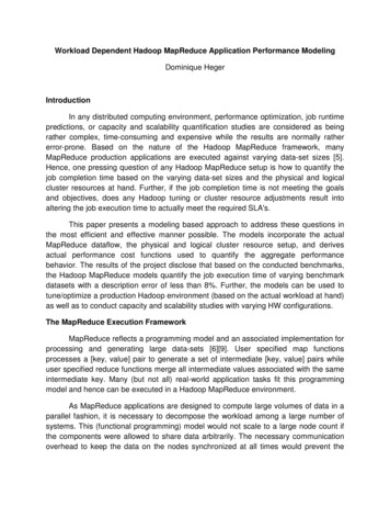
While other Hadoop performance evaluation and quantification studies suggest theusage of an application profiling tool [2],[3],[11], the argument made in this study is thatby solely profiling at the application layer, the level of detail necessary to conductcomprehensive sensitivity studies via the Hadoop models is not sufficient. To illustrate,any IO request at the application layer is potentially transformed at the Linux BIO layer,the Linux IO scheduler, the device firmware, and the disk cache subsystem,respectively. Further, the workload-dependent IO performance behavior is impacted bysome of the Linux specific logical resource parameters such as the setting of the readahead value and/or the IO scheduler being used (see Table 1). To illustrate, the Linuxkernel tends to asynchronously read-ahead data from the disk subsystem if a sequentialaccess pattern is detected. Currently, the default Linux read-ahead block size equals to128KBytes (can be adjusted via blockdev --setra). As Hadoop fetches data in asynchronous loop, Hadoop cannot take advantage of OS' asynchronous read-aheadpotential past the 128KBytes unless the read-ahead size is adjusted on the clusternodes. Depending on the IO behavior of the MapReduce applications, it is rathercommon to increase the read-ahead size in a Hadoop cluster environment.Figure 2: Linux perf Output633.177931 task-clock#0.998 CPUs utilized( 58 context-switches#0.092 K/sec( 0 cpu-migrations#0.000 K/sec( 109,992 page-faults#0.174 M/sec( 1,800,355,879 cycles#2.843 GHz( 290,156,191 stalled-cycles-frontend16.12% frontend cycles idle( 488,353,913 stalled-cycles-backend27.13% backend cycles idle( 2,108,703,053 instructions # 1.17 instructions per cycle0.23 stalled cycles per instructions( 500,187,297 branches# 789.963 M/sec( 761,132 branch-misses# 0.15% of all branches( 29%]0.99%)[66.75%]0.01% )0.01% )0.13% )[83.42%][83.56%][83.42%]To accurately compile the workload profile for the applications, actual mappingfunctions (application primitives onto OS primitives and OS primitives unto the HWresources) are required. This comprehensive code-path based profiling approachfurther allows for conducting sensitivity studies via adjusting logical and physicalsystems components in the model framework at the application, OS, as well as HWlayers. Currently, Hadoop already provides workload statistics such as the number ofbytes read or written (see Figure 3). These stats are periodically transferred to themaster node (with the heartbeat). For this study, the Hadoop code was adjusted withbreakpoints that when reached, triggers the execution of a watchdog program thatmeasures the total execution time for each MapReduce phase and also prompts thecollection of profile and trace data at the application and the OS level. In other words,
for the duration of each phase (see Figure 1), the task execution is profiled and tracedvia the Linux tools strace, perf, blktrace and snapshots via lsof, iotop, ioprofile, and dstatare taken. The breakpoints in the Hadoop code can individually be activated anddeactivated and as the actual trace and profile data is collected outside of the Hadoopframework, the performance impact on the MapReduce execution behavior isminimized.Figure 3: Hadoop Provided Statistics of a Sample WordCount INFOINFOINFOINFOmapred.JobClient: Running job: job 201005121900 0001mapred.JobClient: map 0% reduce 0%mapred.JobClient: map 50% reduce 0%mapred.JobClient: map 100% reduce 16%mapred.JobClient: map 100% reduce 100%mapred.JobClient: Job complete: job 201005121900 0001mapred.JobClient: Counters: 17mapred.JobClient:Job Countersmapred.JobClient:Launched reduce tasks 1mapred.JobClient:Launched map tasks 2mapred.JobClient:Data-local map tasks nt:FILE BYTES READ 47556mapred.JobClient:HDFS BYTES READ 111598mapred.JobClient:FILE BYTES WRITTEN 95182mapred.JobClient:HDFS BYTES WRITTEN 30949mapred.JobClient:Map-Reduce Frameworkmapred.JobClient:Reduce input groups 2974mapred.JobClient:Combine output records 3381mapred.JobClient:Map input records 2937mapred.JobClient:Reduce shuffle bytes 47562mapred.JobClient:Reduce output records 2974mapred.JobClient:Spilled Records 6762mapred.JobClient:Map output bytes 168718mapred.JobClient:Combine input records 17457mapred.JobClient:Map output records 17457mapred.JobClient:Reduce input records 3381After the data collection for the individual MapReduce phases is completed, thedata is post-processed to compile the necessary MapReduce model input parameterssuch as the input key-value size, the map input output data ratio, the reduce inputoutput data ratio, the potential data compression ratios, the memory/cache behavior, theIO activities, as well as the average (per task) cycles per instruction (CPI) demand foreach phase. Some of the performance related parameters expressed via theseperformance-fusion techniques are related to the map, reduce, sort, merge, combine,serialize (transform object into byte stream), partition, compress, and uncompressfunctionalities. In addition, some of major Hadoop tuning parameters and executioncharacteristics (see Table 2) are extracted from the actual Hadoop cluster and used asinput parameters into the models as well.
Hadoop Performance Evaluation and ResultsFor the modeling and sensitivity studies, 2 Hadoop cluster environments were used.First, a 6-node Hadoop cluster that was configured in a 1 JobTracker/NameNode and 5TaskTracker setup. All the nodes were configured with dual-socket quad-core IntelXeon 2.93GHz processors, 8GB (DDR3 ECC 1333MHz) of memory, and were equippedwith 4 1TB 7200RPM SATA drives each. Second, a 16-node Hadoop cluster, with 1node used as the JobTracker, 1 node as the NameNode, and 14 nodes asTaskTrackers, respectively. All the nodes in the larger Hadoop framework wereconfigured identically to the 6-node execution framework, except on the IO side. Eachnode in the larger Hadoop setup was equipped with 6 1TB 7200RPM SATA drives. Forboth Hadoop cluster setups, the cluster interconnect was configured as a switched GigEnetwork. Both clusters were powered by Ubuntu 12.04 (kernel 3.6) and CDH4 Hadoop.For all the benchmarks, replication was set to 3. The actual Hadoop performanceevaluation study was executed in 6 distinct phases:1. Establish the Model profiles (as discussed in this paper) for the 3 Hadoopbenchmarks TeraSort, K-Means, and WordCount on the 6-node Hadoop cluster.All 3 benchmarks disclose different workload behaviors and hence reflect a goodmix of MapReduce challenges (see Figure 4). For these benchmark runs, thedefault Java, Hadoop, and Linux kernel parameters were used (aka no tuningwas applied). In other words, the HDFS block size was 64MB, the Java Heapspace 200MB, the Linux read-ahead 256KB, and 2 Map and 2 Reduce slots wereused per node.2. Use the established workload profiles in conjunction with the HW profiles tocalibrate and validate the Hadoop models. Execute the simulation and determinethe description error (delta empirical to model job execution time).3. Use the developed Hadoop models to optimize/tune the actual workload basedon the physical and logical resources available in the 6-node Hadoop model. Inthis stage, the methodology outlined in [10] was used to optimize/tune theHadoop environment via the models.4. Apply the model-based tuning recommendations to the 6-node cluster. Rerun theHadoop benchmarks and establish the description error (delta tuned-empirical totuned-model job execution time).5. Use the tuned-model baseline to conduct a scalability analysis, scaling theworkload input (increase the problem size) and mapping that new workload ontoa 16-node Hadoop cluster that is equipped with 6 instead of 4 SATA drives perTaskTracker.6. Execute the actual Hadoop benchmarks on the 16-node Hadoop cluster (with thetuning and setup recommendations made via the model). Establish the
description error tuned-scaled-empirical to tuned-scaled-model job executiontime.Figure 4: Hadoop Benchmark Applications (Figure courtesy of Intel)In phase 1, all 3 Hadoop benchmarks were executed 20 times on the smallHadoop cluster. During the benchmark runs, Hadoop and Linux performance data wascollected. The Linux performance tools such as perf and blktrace added anapproximately 3% additional workload overhead onto the cluster nodes. That overheadwas taking into consideration while running the models. After all benchmarks wereexecuted, a statistical analysis of the benchmark runs revealed a CV (coefficient ofvariation) of less than 4% and hence the collected sample sets are considered asproducing repeatable benchmark data. All the collected Hadoop and Linux data waspost-processed and utilized as input into the Hadoop models. In phase 2, the calibratedmodels were used to simulate the 3 Hadoop benchmark runs. The results of the first setof simulation runs disclosed a description error of 5.2%, 6.4%, and 7.8% for theTeraSort, K-Means, and WordCount benchmarks, respectively. In phase 3, the tuningmethodology outlined in [10] was used to optimize the actual workload onto theavailable physical and logical systems resources. Figure 5 shows the modeled nontuned benchmark execution time for the TeraSort, scaling the number of nodes from 4to 8. Figure 6 discloses the tuned TeraSort execution time. By applying the tuningmethodology, the aggregate TeraSort execution time for the 5 TaskTracker setup wasimproved (lowered) by a factor of 2.8.Figure 5: TeraSort - Default Hadoop Parameters, 4GB Inpu
a holistic, modeling based performance and scalability evaluation framework. The Hadoop models incorporate the physical and logical systems setup of the underlying Hadoop cluster (see Table 1), the major Hadoop tuning parameters (see Table 2), as well as the workload profile abstraction of the MapReduce application. As with any