Transcription
HindawiMathematical Problems in EngineeringVolume 2021, Article ID 6636367, 14 pageshttps://doi.org/10.1155/2021/6636367Research ArticleMultistep Prediction of Bus Arrival Time with the RecurrentNeural NetworkZhi-Ying Xie,1,2 Yuan-Rong He,1,2 Chih-Cheng Chen ,3,4 Qing-Quan Li,5and Chia-Chun Wu 61School of Computer and Information Engineering, Xiamen University of Technology, Xiamen 361024, ChinaDigital Fujian Institute of Natural Disaster Monitoring Big Data, Xiamen, Fujian 361024, China3Department of Automatic Control Engineering, Feng Chia University, Taichung 40724, Taiwan4Department of Aeronautical Engineering, Chaoyang University of Technology, Taichung 413, Taiwan5Shenzhen Key Laboratory of Spatial Smart Sensing and Services, Shenzhen University, Shenzhen 518060, China6Department of Industrial Engineering and Management, National Quemoy University, Kinmen 892, Taiwan2Correspondence should be addressed to Chih-Cheng Chen; ccc@gm.cyut.edu.tw and Chia-Chun Wu; ccwu0918@nqu.edu.twReceived 30 October 2020; Revised 3 January 2021; Accepted 18 February 2021; Published 12 March 2021Academic Editor: Bosheng SongCopyright 2021 Zhi-Ying Xie et al. This is an open access article distributed under the Creative Commons Attribution License,which permits unrestricted use, distribution, and reproduction in any medium, provided the original work is properly cited.Accurate predictions of bus arrival times help passengers arrange their trips easily and flexibly and improve travel efficiency.Thus, it is important to manage and schedule the arrival times of buses for the efficient deployment of buses and to ease trafficcongestion, which improves the service quality of the public transport system. However, due to many variables disturbing thescheduled transportation, accurate prediction is challenging. For accurate prediction of the arrival time of a bus, this researchadopted a recurrent neural network (RNN). For the prediction, the variables affecting the bus arrival time were investigatedfrom the data set containing the route, a driver, weather, and the schedule. Then, a stacked multilayer RNN model was createdwith the variables that were categorized into four groups. The RNN model with a separate multi-input and spatiotemporalsequence model was applied to the data of the arrival and leaving times of a bus from all of a Shandong Linyi bus route. Theresult of the model simulation revealed that the convolutional long short-term memory (ConvLSTM) model showed thehighest accuracy among the tested models. The propagation of error and the number of prediction steps influenced theprediction accuracy.1. IntroductionThe rapid and continuous development of China has led to anincrease in the number of vehicles. The National Bureau ofStatistics of China announced that the number of privatelyowned vehicles reached 261.5 million in 2019 with 21.22million vehicles increased in a year. 96 cities in China hadmore than one million registered vehicles [1]. The rapidincrease of vehicles causes traffic congestion, parking problems, and environmental pollution. Public transportationaffords a larger number of passengers and alleviates suchproblems. Mass transportation consumes less energy andemits less amount of pollutants than private transport.Therefore, urban planning puts a priority on publictransportation. New technologies such as bus rapid transit(BRT) and driverless bus have been developed significantlywith huge investment to support the public transportationsystem. However, a trip by bus takes a relatively long time andis not punctual, which makes people avoid it. Encouragingpeople to use buses more often requires optimized bus routesand punctuality of bus operation [2, 3]. However, the absenceof an accurate operation schedule often causes long waitingtimes and bus bunching on the same route. For the punctualoperation of the public buses, the bus schedule needs to beoptimized, which needs an accurate prediction of the arrivaltime of buses on a route accurately. This not only meets thedemand of ordinary passengers who want to know the arrivaltimes of a bus at boarding stations but also optimizes the
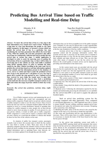
2intelligent bus scheduling system and improves the operationefficiency of the bus company.Several neural networks have been used to predict thearrival time of a bus: non-RNN network, RNN with the timeseries, and temporal and spatial RNN network. Severalstudies adopted non-RNN networks for predicting bus arrival and operation times using (1) MapReduce-basedclustering with K-means [4], (2) a backpropagation (BP)neural network model [5], (3) a particle swarm algorithm[6], (4) a wide-depth recursive (WDR) learning model [7],and (5) RNN with the time series such as long short-termmemory (LSTM) [8]. Models with LSTM processed thehistorical data of the global position system (GPS) and busstop locations with the influence of different routes, drivers,weather conditions, time distribution [9], heterogeneoustraffic flow, and real-time data [10–12]. The temporal andspatial RNN network with ConvLSTM or a spatiotemporalproperty model (STPM) was originally used to predict theprecipitation [13]. However, it was also used for predictingbus arrival times based on the total operation time of a buson a route, waiting and on-board times, transfer locationwait times [14–16], and multilane short-term traffic flow [17]and for creating the multitime step deep neural network [18].The bus is running on fixed lines with fixed stations. Thespatial relationship between its stations determines the arrivaltimes in the time series. Thus, this study used an RNN topredict the arrival time of a bus. A route of a bus has 30–40bus stations in general. Arrival time prediction includes thetime prediction of each station along the way from the startingto the finishing stop, the arrival times at subsequent stations,and the arrival time of the nearest vehicle to a station. Thisstudy first analyzed the bus arrival time. Based on the analysis,the input eigenvectors of a neural network were defined, andthen, seven RNN models for predicting the arrival time fromfour categories were tested. Then, the proposed model wastrained by the measured data of arrival and departure times ofthe buses in a route of Linyi, Shandong Province. Then, themultistep prediction of the arrival time was carried out.This paper is organized as follows. Section 2 describes thetheoretical background and introduces the recurrent neuralnetwork. Section 3 describes the pretreatment and analysisof data. Section 4 discusses the analysis result of the RNNmodel. Finally, Section 5 concludes this study.2. Theoretical BackgroundA recurrent neural network (RNN) [19] has a feedbackstructure that processes sequential data for time-seriesprediction or classification. RNN is widely used in variousapplications, and new models using it have been suggestedsuch as LSTM, GRU, and ConvLSTM. According to the datain this study, we divided the prediction into four categoriesand adopted a multistep prediction for bus arrival times. Thetime-series input data is essential for the prediction withoptimal feature extraction and memory efficiency. The datais processed in an RNN with internal feedback and feedforward connection, which retain and reflect the state ormemory of a long context window [20]. The RNN suffersfrom a common disadvantage of the gradient disappearanceMathematical Problems in Engineering(gradient vanishing) and gradient explosion problem[21–23], which results in limited applications due to trainingproblems. To solve the problems, Hochreiter et al. [24]proposed and continued improving LSTM for differentapplications [25, 26]. LSTM specializes in memorizing longsequences and effectively avoiding the problem of gradientdisappearance. Hidden layers of LSTM use memory blocksthat store the previous sequence information, while increasing the performance of three gates: input, output, andforget gates. These control the sequence information formemory. The gated recurrent unit (GRU) [27] is a modestlysimplified LSTM. GRU combines the forget and input gateinto an update gate and the cell and hidden state. A modelwith GRU is simpler and has less activation function andoutput computation than the standard LSTM model.2.1. Pure LSTM and Pure GRU Model. Figure 1 shows thehidden units of LSTM which are replaced by memory blocks.Calculating ct and ht requires the following equations:it σ Wi Xt Ui ht 1 bi (Input gate),ft σ Wf Xt Uf ht 1 bf (Forget gate),ot σ Wo Xt Uo ht 1 bo (Output gate),(1) ct tanh Wc Xt Uc ht 1 bc (New memory cell),ct ft ct 1 it ct (Memory cell),ht ot tanh ct .In these equations, Hadamard product is the multiplication of the corresponding elements in the operationmatrix, Wi , Wf , Wo , and Wc are the weights of Xt , Ui , Uf ,Uo , and Uc are the weights of ht 1 , bi , bf , bo , and bc are thebias conditions, σ is the sigmoid function, and tanh is thehyperbolic tangent function.Figure 2 shows the GRU. There is only one hidden state htin GRU. Through the linear transformation of the inputtensor and hidden state, the weighted sum of the hidden stateinflow is calculated with equations (2) and (3). The lineartransformation for rt , ht 1, and the input tensor is combinedwith the activation function of equation (4) to calculate theupdated value of the hidden state. The mixed weight forcalculation of the implicit state in the previous step is shownin equation (5). The final output ht is the same as LSTM.Compared with LSTM, there is one less activation functioncalculation and output calculation as well as the final hiddenstate update, so the calculation is relatively simple.zt σ Wz Xt Uz ht 1 bz (Update gate),(2)rt σ Wr Xt Ur ht 1 br (Reset gate),(3)h t tanh Wh Xt rt Uh ht 1 bh (New memory cell),(4)ht 1 zt h t zt ht 1 .(5)
Mathematical Problems in Engineering3ytct 1 cttanhft itσσc t otσtanhht 1employed. Stacking four LSTMs had hidden units in 256,128, 64, and 32 layers, respectively. Figure 5(a) shows thediagram of the stacking models. There is also a two-wayLSTM composition, in which the forward and backwardconnections also employ a reverse projection function,which is suitable in our case to verify arrival time predictions. Figure 5(b) shows the diagram of the bidirectionalnetwork models.ht2.4. Spatiotemporal Time-Series Model. The bus operation isin a space-time domain although there are little changes inthe spatial dimension for an operation in the fixed route. AsConvLSTM processes the data of time and space, it integrates a convolution of time and space into calculating eachgate of LSTM. The following equations are used for thecalculation:XtFigure 1: LSTM memory cell structure.yt ht 1 1–ztrtσ σ ht htit σ Wi Xt Ui ht 1 bi (Input gate),(6)ft σ Wf Xt Uf ht 1 bf (Forget gate),(7)ot σ Wo Xt Uo ht 1 bo (Output gate),(8)tanh ct tanh Wc Xt Uc ht 1 bc (New memory cell),(9)XtFigure 2: GRU unit structure.Figure 3 illustrates a pure network model of LSTM andGRU. The input layer has the sequence of the arrival timeseries input, and the other two layers use a fully connectedprediction network. Input and output data are 3D tensorswith a shape [?, 41, 1] (“? ”means that a dimension can haveany length).These models use a single layer of LSTM and GRU. In theinput layer, variables are, such as route, direction, vehiclemodel, and driver, also regarded as a part of the time sequence.ct ft ct 1 it ct (Memory cell),(10)ht ot tanh ct .(11)A ConvLSTM network with batch normalization (BN)consists of a specification and flattening layer and a prediction network. Figure 6 shows the diagram of the networkthat has a long training time and many parameters in morethan five dimensions. This network is appropriate to processtime-series data with spatial properties such as bus arrivaltimes with high accuracy.3. Pretreatment and Analysis of Data2.2. Multi-Input Model Separated by Time Series. As thevariable is not sensitive to any specific ordering, the RNNcannot process it alone. However, a BP network can processthrough a connection layer. Thus, the integration of RNNand BP was used for the prediction network (Figure 4).The integrated network was in accordance with thecharacteristics of the input data. A two-part network usedthe time series-related input data such as route number,driver, departure time, and route length for LSTM processing. Through a connection layer, the prediction layerwas processed. Since time series input data became shortereven with the addition of LSTM, the total trainable parameters were not significantly increased compared withpure LSTM.2.3. LSTM Stacking Model. To achieve better accuracy of theprediction than a single layer, a multilayer LSTM was3.1. Data Characteristics. A bus was equipped with a devicethat included a GPS and data communication module. Thedevice transmitted data to a bus scheduling system. Table 1shows the data structure of the reporting system.The data of arrival and departure of a bus at a bus stopconsists of route, speed, arrival and departure time, coordination, and driver’s number. For obtaining the Lassovariable correlation [8], the bus number, number of busstops, days in the week, distances between bus stops, arrivaland departure times, and weather were included, too. Thevariables were grouped into two: dynamic and static variables [14]. The dynamic variables include driving timesbetween bus stops, staying times, and weather, while thestatic variables include a route, direction, vehicle model,driver, arrival and departure times, days of the week, holidays, and working days. We selected variables related to theroute and the arrival times at the previous stops as the input
4Mathematical Problems in EngineeringInput layerinput:[(?, 41, 1)]output:[(?, 41, 1)]input:(?, 41, 1)output:(?, 64)GRUDenseDenseinput:(?, 64)output:(?, 32)input:(?, 32)output:(?, 33)Input layerLSTMDenseDenseinput:[(?, 41, 1)]output:[(?, 41, 1)]input:(?, 41, 1)output:(?, 64)input:(?, 64)output:(?, 32)input:(?, 32)output:(?, 33)Figure 3: A pure LSTM and pure GRU network model.Input layerLSTMLSTMinput:[(?, 32, 1)]output:[(?, 32, 1)]input:(?, 32, 1)output:(?, 32, 64)input:(?, 32, 64)output:(?, 32)ConcatenateDenseDenseInput feature: [route no, direction, bus no, driver no,departure hours, departure minutes, days of the week,holidays, distance, and weather (xt k , . . . , xt )]Output prediction series: ( xt k , . . . , 0, xt 1 , . . . , xt n )Input layerDenseinput:[(?, 9)]output:[(?, 9)]input:(?, 9)output:(?, 16)input:[(?, 16), (?, 32)]output:(?, 48)input:(?, 48)output:(?, 32)input:(?, 32)output:(?, 33)Figure 4: An LSTM-BP integrated network model.features to predict the arrival time at a bus stop. Input andoutput features are as follows:where xt is the difference of the arrival time between thecurrent station and the previous station.3.2. Data PreprocessingStep 1. Generating a Sample DatasetAccording to the data in Section 3.1, an arrival timeseries was obtained from the data of arrival and departuretimes of a bus at a bus stop. For the convenience of calculation, the difference of the arrival times between two busstops was calculated in seconds. Table 2 shows the exampleof the dataset. The existing sequence data are 120, 220, 250,and 260 which correspond to four bus stops A, B, C, andD. This means that 120 s is needed for a bus to drive from thestarting location to A, 220 s from A to B, 250 s from B to C,and 260 s from C to D. When the bus arrives at C, theprediction of the arrival time to D is only needed. The inputsequence is the sequence of all arrival times from the startinglocation to C, and the output sequence includes 260 s from Cto D and the backward sequence from C to the startinglocation. The length of the input sequence is shorter thanthat of the output sequence as it only needs to predict thetime to the finishing location of a bus. When predicting thetime to the finishing location, it only needs to know thesequences before it. When the bus arrives at a bus stop
Mathematical Problems in EngineeringInput layerLSTMLSTMLSTMLSTMDenseDense5input:[(?, 41, 1)]output:[(?, 41, 1)]input:(?, 41, 1)output:(?, 41, 256)input:(?, 41, 256)output:(?, 41, 128)input:(?, 41, 128)output:(?, 41, 64)input:(?, 41, 64)output:(?, 32)input:(?, 32)output:(?, 32)input:(?, 32)input:[(?, 41, 1)]output:[(?, 41, 1)]Input layerBidirectional (LSTM)Bidirectional (LSTM)Denseinput:(?, 41, 1)output:(?, 41, 128)input:(?, 41, 128)output:(?, 64)input:(?, 64)output:(?, 32)input:(?, 32)output:(?, 33)Denseoutput:(?, 33)Figure 5: (a) A LSTM stacking model. (b) A bidirectional LSTM model.between the starting and finishing location, for a consistentsequence length, the time to the previous bus stop is input as0.Figure 7 shows the time-series data of real arrivaltimes. The blue and orange line is for the input andoutput sequence, respectively. The sequence has thepredicted times of 0 at the current bus stop. An outputsequence has negative numbers to maintain the correctness of the inverted time from the starting location tothe bus stop.Step 2. Dataset NormalizationThe variables had different dimensions and units whichaffected the results of data analysis. Thus, normalization wasnecessary to eliminate the differences. Standardizing withthe Z-score and the minimum-maximum values were usedso that the final values were ranged between 0-1. Theequation for standardization is as follows:xnorm x min(x).max(x) min(x)(12)
6Mathematical Problems in Engineeringinput:[(?, 41, 1, 1, 1)]250output:[(?, 41, 1, 1, 1)]200ConvLSTM2Dinput:(?, 41, 1, 1, 1)output:(?, 41, 1, 1, 41)Batch normalizationFlatteninput:(?, 41, 1, 1, 41)output:(?, 41, 1, 1, 41)input:(?, 41, 1, 1, 41)output:(?, 1681)Arrivate time (s)Input layer150100500–50–100–15005101520Bus stationDenseinput:(?, 1681)output:(?, 32)input:(?, 32)output:(?, 33)Figure 6: ConvLSTM network model.Table 1: The data structure from a bus.No.1234567891011121314151617NameRoute noRoute nameRoute subnoUp downBus noSpeeddatatime indriver nobusstop nobusstop namebusstop lngbusstop latbusstop serialbusstop typepack datetimeinform typenetpack tringDoubleDoubleIntIntStringIntIntRemarksRoute numberRoute nameRun method no.Direction on routeVehicle numberSpeedEntry timeDriver numberSite numberSite nameSite longitudeSite latitudeSite serial numberSite typeOutbound timeInform modeEntry modeTable 2: Examples of the arrival time-series dataset format.Input sequence(120, 220, and 250)(120, 220, and 0)(120, 0, and 0)Output sequence( 120, 220, 0, and 260)( 120, 0, 250, and 260)(0, 220, 250, and 260)Z-score standardization uses the mean and standarddeviation of the data and is calculated as follows:30Figure 7: A diagram of the input and output sequence generated bythe time-series data of arrival times.xnorm Dense25x μ,σ(13)where µ is the mean and σ is the standard deviation of thedata.In this paper, after sorting the vehicle number and drivernumber on the route, the sorted sequence was used as theinput data and normalized by equation (7). The routenumber, route direction, departure time (hh:mm), days ofthe week, holidays, distances from the starting location,weather, and other information were normalized, and theirarrival time series were processed by equation (8).4. Analysis Result of the RNN Model4.1. Dataset. The experiment was based on the data collectedfrom March 28 to June 28, 2020, in Linyi, ShandongProvince. The data was obtained from buses that ran onroute no. 30 which had 36 bus stops (Figure 8). TensorflowGPU 2.0 was used for data processing and algorithm creation. The numbers of the dataset were 122,336 after pretreatment, 78,303 in the training set, 19,590 in theverification set, and 24,443 in the test set.4.2. Training the RNN Prediction Model. Seven networkmodels were designed, trained, verified, and tested by usingthe preprocessed dataset. Pure LSTM and GRU were RNNmodels. LSTM-BP and GRU-BP were multiple input modelswith variable features separated from the time series. Bidirectional LSTM (LSTM-Bi) and LTSM-Stack were LSTMstack models. ConvLSTM was a spatiotemporal sequencemodel. Table 3 shows a model structure and a comparison ofthe parameters of the RNN network. Pure GRU had thesmallest number of the parameter, while the stack model hadthe largest number.The loss function selected the average absolute error(MAE) which was the difference between the prediction andreal value. All network parameters were updated using theAdam optimization algorithm. The Adam algorithm performs first-order optimization. The first- and second-orderoptimizations were used for a dynamic design of independent adaptive learning rates for different parameters. The
Mathematical Problems in Engineering74325678910221821 20 1917 16 15 14131112232430 29 282627253132333435Figure 8: Linyi city’s 30 bus routes and site distribution.Table 3: Seven RNN network model structures and their parameters.ClassificationType ofnetworkPure GRUPure RNNPure LSTMGRU-BPMulti-input hybridmodelLSTM-BPLSTM-BiStacking modelsLTSM-StackType of layerOutput sequenceGRUDenseDenseLSTMDenseDenseInput layerInput layerGRUDenseGRUConcatenateDenseDenseInput layerInput al (LSTM(64))Bidirectional e, 41, 64) (None, 32)(None, 33)(None, 64)(None, 32)(None, 33)[(None, 32, 1)][(None, 9)](None, 32, 64)(None, 16)(None, 32)(None, 48)(None, 32)(None, 33)[(None, 32, 1)][(None, 9)](None, 32, 64)(None, 16)(None, 32)(None, 48)(None, 32)(None, 33)Number 08015681089001689616012416015681089(None, 41, 128)33792(None, 64)41216(None, 32)(None, 33)(None, 41, 256)(None, 41, 128)(None, 41, 64)(None, 32)(None, 32)(None, 33)20801089264192197120494081241610561089Total number ofparameters15,00920,06525,08932,12978,177525,281
8Mathematical Problems in EngineeringTable 3: Continued.Type ofnetworkClassificationType of layerConvLSTM2DSpace-time modelBNConvLSTMNumber ofparametersOutput sequenceFlattenDenseDense(None, 41, 1, 1,41)(None, 41, 1, 1,41)(None, 1681)(None, 32)(None, 33)621561640.200.80.180.70.160.60.14MAECosine similarityTraining and validation ,2330538241089Training and validation cosine similarity0Total number ofparameters10000200400EpochTraining similarityValidation similarity6008001000EpochTraining lossValidation lossFigure 9: Loss function and accuracy diagram during training.estimations were better than the traditional gradient descentmethod. Since the output was a time series, cosine similaritywas used to determine the accuracy.Figure 9 shows the training loss and accuracy when anepoch is 1000, a batch is 100, and a verification set is 20% ofthe training set. As the seven models show similar MAEs,only the training output of the ConvLSTM model was selected. In the process of training, the trend of training andvalidation data is consistent, and there is no fitting case. Thesuper parameters of the selected model are suitable, too. Asseen from Figure 10, the pure GRU had fewer trainingparameters and less training time than pure LSTM. TheLSTM-Bi doubled the number of parameters and trainingtime than the pure LSTM. The LSTM-Stack had five timesmore parameters than other models, but less training timethan the ConvLSTM. The ConvLSTM had the longesttraining time, 5.8 times more parameters, and 12 timeslonger training time than the pure LSTM.4.3. Analysis of Results. The test set was used to predict thetraining model, and the predicted arrival times are shown inTable 4.The fitting degree of the real and the predicted value inTable 4 shows that the ConvLSTM provides the best prediction. The multi-input hybrid model, which separates theparameters from the time series, not only increased thenetwork complexity but also reduced the prediction accuracy. Table 5 shows the statistics of the prediction results bythe seven models. MAE, RMSE, MAE, COS, number oftraining parameters, and time were used to quantitativelyevaluate the seven network models. The prediction accuracywas improved from the pure LSTM to the ConvLSTM, asshown in Figure 11.The results reveal the following:(1) The GRU was more efficient than the LSTM modelwith fewer parameters and considerable accuracy(2) The LSTM models except the ConvLSTM had moreparameters and higher network accuracy than othermodels(3) The dataset property did not influence the results ofthe models but the complexity of the models(4) The ConvLSTM showed the highest accuracy as itprocessed the data of time and space, which indicated the need to include the space-related propertiesIn the process of arrival time-series prediction, the arrival times at subsequent bus stops were based on those atthe previous bus stops. The ConvLSTM network model wasselected to analyze the prediction accuracy through one- andtwo-step prediction and total time prediction.
100000Training time (s)Trainable parametersMathematical Problems in BPGEU–BPPure LSTMPure GRU0RNN modelTrainable parametersTraining time (s)Figure 10: Comparison of training parameters and times of seven RNN models.Table 4: List of arrival times predicted by the seven models.Network classificationNetwork modelPredicted arrival time seriesPure LSTMArrival time (s)2001000–100–20005101520Bus station2530101520Bus station2530ActualPredictedPure RNN250Pure GRUArrival time (s)200150100500–50–10005ActualPredicted
10Mathematical Problems in EngineeringTable 4: Continued.Network classificationNetwork modelPredicted arrival time series250LSTM-BPArrival time (s)200150100500–5005101520Bus station2530ActualPredictedMulti-input hybrid model200GRU-BPArrival time 20Bus station2530
Mathematical Problems in Engineering11Table 4: Continued.Network classificationNetwork modelPredicted arrival time series200Arrival time (s)150LSTM-Bi100500–50–10005101520Bus station2530101520Bus station2530101520Bus station2530ActualPredictedStacking models200Arrival time dicted100Space-time modelArrival time ctedTable 5: Statistics of the prediction results of seven models.ModelPure LSTMPure 0.9595MAE: mean absolute error; RMSE: root mean square error; COS: cosign similarity.Trainable ,233Training time (s)512058206812788691261317261773
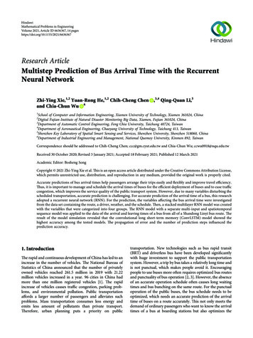
12Mathematical Problems in �BPPure LSTMPure GRU17RNN modelCOSMAEFigure 11: Prediction accuracies of the seven models.Two step prediction vs testRMSE: 63.606052Mean: 27.946125One step prediction vs testRMSE: 42.791447Mean: 4002000–100–200–200–300050001000015000Test sample set0200001 step fferenceTotal time prediction vs testRMSE: 242.42374Mean: 002 step biasMean(a)01000015000Test sample set1000015000Test sample t prediction2001 step bias2 step biasTotalTotalMean(c)(d)Figure 12: Multistep prediction comparison chart. (a) One step. (b) Two step. (c) Total. (d) Histogram.300400
Mathematical Problems in EngineeringFigure 12 shows the test sample set on the x-axis and thedifference between the predicted and real values on the yaxis. The mean and RMSE were calculated from the meanvalues and mean square deviation of the differences. Theone-step prediction had the highest accuracy, and the totaltime prediction (multistep prediction) showed the lowestaccuracy. The regularity in the histogram of Figure 12 revealsthat the one-step prediction has the smallest deviation andthe highest error, which is related to the accumulation andpropagation of errors in the prediction of the arrival times ofthe subsequent bus stops.5. ConclusionThe public transport system is a complex system with a highdegree of uncertainty. The system is understood as a multistep prediction problem in which uncertainty leads to poorprediction accuracy. This paper first analyzed the mainvariables affecting this uncertainty, and then, the variablessuch as route, direction, vehicle, driver, departure hour,departure minute, day of the week, holiday, distance fromthe starting location, and weather were selected. The arrivaltime series before the current bus stops was also selected.These variables fully reflected the impact on the arrival timeseries prediction. Among RNN networks for time-seriesanalysis, we processed the data by using seven differentnetwork models in four different types of networks.We analyzed and compared the predictive power of theseven RNN models with the variables and parameters in themeasured dataset. We noticed an improvement in predictionaccuracy by adding variables in one- and two-step predictionmodels, but not in the multistep (total time prediction)model. The multistep model increased the network complexity only. The ConvLSTM showed the highest predictionaccuracy with spatiotemporal data. The statistics of one-,two-, and multistep prediction showed that the accumulation and propagation of the sequence prediction errorcaused more steps and a large deviation of the predictedtime. The accurate bus arrival time prediction encouragesmore people to use buses for transportation and allowsoperating companies to optimize bus schedules for increasing the efficiency of their operation. This also improvesthe traffic condition in cities.Accurate bus arrival informa
consists of route, speed, arrival and departure time, coor-dination, and driver's number. For obtaining the Lasso variable correlation [8], the bus number, number of bus al and departure times, and weather were included, too. e variables were grouped into two: dynamic and static vari-