Transcription
DISCOVERING STATISTICS USING SPSSChapter 19: Categorical outcomes: chi-squareand loglinear analysisLabcoat Leni’s Real ResearchThe impact of sexualized images on women’s self-evaluationsProblemDaniels, E., A. (2012). Journal of Applied Developmental Psychology, 33, 79–90.Women (and increasingly men) are constantly bombared with images of‘idealized’ women in the media and there is a growing concern abouthow these images affect our perceptions of ourselves. Daniels (2012)conducted an interesting study in which she showed young womenimages of successful female athletes (e.g., Anna Kournikova) that wereeither images of them playing sport (performance athlete images) orimages of them posing in bathing suits (sexualized images). Participantscompleted a short writing exercise after viewing these types of images. Each participant sawonly one type of image, but several examples. Daniels then coded these written exercisesand identified themes, one of which was whether women commented on their ownappearance or attractiveness. Daniels hypothesized that women who viewed the sexualizedimages (n 140) would self‐objectify (i.e., this theme would be present in what they wrote)more than those who viewed the performance athlete pictures (n 117, despite what theparticipants section of the paper implies). These are the frequencies:Performance athletesSexualized athletesTheme Present2056Theme Absent9784Total117140Labcoat Leni wants you to enter these data in SPSS and test Daniel’s hypothesis thatthere is an association between the type of image viewed, and whether or not the womencommented on their own appearance/attractiveness in their writing exercise ( Daniels(2012).sav).SolutionBecause the frequency data have been entered into SPSS, we must tell the computer thatthe variable Self Evaluation represents the number of cases that fell into a particularcombination of categories. To do this, access the Weight Cases dialog box by selecting. Selectand then drag the variable in which the number of casesis specified (in this case Self Evaluation) to the box labelled Frequency variable (or click on). This process tells the computer that it should weight each category combination by thePROFESSOR ANDY P FIELD1
DISCOVERING STATISTICS USING SPSSnumber in the column labelled Self Evaluation. Your completed dialog box should look likeFigure Figure 1.Figure 1Next, select. First, drag one of the variables ofinterest from the variable list to the box labelled Row(s) (or select it and click on ). For thisexample, I selected Type of Picture to be the rows of the table. Next, drag the other variableof interest (Was Theme Present or Absent in what participant wrote) to the box labelledColumn(s) (or select it and click on ). If you click ona dialog box appears in whichyou can specify various statistical tests. Select the chi‐square test, the contingencycoefficient, phi and lambda and then click on. If you click ona dialog boxappears in which you can specify the type of data displayed in the crosstabulation table. It isimportant that you ask for expected counts because this is how we check the assumptionsabout the expected frequencies. It is also useful to have a look at the row, column and totalpercentages because these values are usually more easily interpreted than the actualfrequencies and provide some idea of the origin of any significant effects. There are twoother options that are useful for breaking down a significant effect (should we get one): (1)we can select a z‐test to compare cell counts across columns of the contingency table (bychecking), and if we do we should use a Bonferroni correction (check); and (2) select standardized residuals. Once these options havebeen selected, click onto return to the main dialog box. From here you can click onto compute Fisher’s exact test if your sample is small or if your expected frequenciesare too low. Select the Exact test option; we don’t really need it for these data, but it will bea useful way to see how it is used. Click onto return to the main dialog box and thenclick onto run the analysis (your completed dialog boxes should look like those inFigure Figure 2).PROFESSOR ANDY P FIELD2
DISCOVERING STATISTICS USING SPSSFigure 2PROFESSOR ANDY P FIELD3
DISCOVERING STATISTICS USING SPSSOutputOutput 1First, let’s check that the expected frequencies assumption has been met. We have a 2 2table, so all expected frequencies need to be greater than 5. If you look at the expectedcounts in the contingency table, we see that the smallest expected count is 34.6 (for womenwho saw pictures of performance athletes and did self‐evaluate). This value exceeds 5 andso the assumption has been met.The other thing to note about this table is that because we selected Compare columnproportions our counts have subscript letters. For example, in the row labelled PerformanceAthletes the count of 97 has a subscript letter a and the count of 20 has a subscript letter b.These subscripts tell us the results of the z‐test that we asked for: columns with differentsubscripts have significantly different column proportions. We need to look within rows ofthe table. So, for Performance Athletes the columns have different subscripts as I justexplained, which means that proportions within the column variable (i.e., Was the themepresent or absent in what they wrote?) are significantly different. The z‐test compares theproportion of the total frequency of the first column that falls into the first row against theproportion of the total frequency of the second column that falls into the first row. So, of allthe women who did self‐evaluate (theme present), 26.3% saw pictures of performanceathletes, and of all the women who didn’t self‐evaluate (theme absent), 53.6% saw picturesof performance athletes. The different subscripts tell us that these proportions aresignificantly different. Put another way, the proportion of women who self‐evaluated afterseeing pictures of performance athletes was significantly less than the proportion who didn’tself‐evaluate after seeing pictures of performance athletes.If we move on to the row labelled Sexualized Athletes, the count of 84 has a subscriptletter a and the count of 56 has a subscript letter b; as before, the fact they have differentletters tells us that the column proportions are significantly different. The proportion ofPROFESSOR ANDY P FIELD4
DISCOVERING STATISTICS USING SPSSwomen who self‐evaluated after seeing sexualized pictures of female athletes (73.7%) wassignificantly greater than the proportion who didn’t self‐evaluate after seeing sexualizedpictures of female athletes (46.4%).As we saw earlier, Pearson’s chi‐square test examines whether there is an associationbetween two categorical variables (in this case the type of picture and whether the womenself‐evaluated or not). The value of the chi‐square statistic is 16.057. This value is highlysignificant (p .001), indicating that the type of picture used had a significant effect onwhether women self‐evaluated.Underneath the chi‐square table there are several footnotes relating to the assumptionthat expected counts should be greater than 5. If you forgot to check this assumptionyourself, SPSS kindly gives a summary of the number of expected counts below 5. In thiscase, there were no expected frequencies less than 5, so we know that the chi‐squarestatistic should be accurate.Output 2The highly significant result indicates that there is an association between the type ofpicture and whether women self‐evaluated or not. In other words, the pattern of responses(i.e., the proportion of women who self‐evaluated to the proportion who did not) in the twopicture conditions is significantly different.Below is an excerpt from Daniels’s (2012) conclusions:PROFESSOR ANDY P FIELD5
Underneath the chi‐square table there are several footnotes relating to the assumption that expected counts should be greater than 5. If you forgot to check this assumption yourself, SPSS kindly gives a summary of the number of expected counts below 5. In this case, there were no expected frequencies less than 5, so we know that the chi .