Transcription
Swaptions pricing under the single factorHull-White Model through the Analyticalformula and Finite Difference MethodsVictor Lopez Lopez1Jan Röman21 Corresponding author, student of the Master of Science in Mathematics with focus inFinancial Engineering at Mälardalen University.2 Division of Applied Mathematics, Mälardalen University.
AbstractDue to the interesting financial moment we are living, my motivations to writethis Master thesis has mostly been the behavior of interest rates and modelsthat can be used predict them. Thus, in this dissertation I have presented theHull-White model and the way to calibrate it against market data so it can beused to price interest rate derivatives. The reader can find both theoretical andpractical presentations and examples along with the code to program them byhim/herself.I would like to take advantage of the situation and thank Jan Röman as Ihave relied through all this work on his lessons at Mälardalens University. Thus,I would like to refer the reader to his work in the references [1] and [7] whenseeking for any deeper knowledge in this topic.
Contents1 Introduction42 Interest rate derivatives2.1 Bonds, FRN and FRA . . . . .2.2 Swaps . . . . . . . . . . . . . .2.3 Swaptions . . . . . . . . . . . .2.4 Interest rate derivatives pricing2.5 Martingale modeling . . . . . .2.5.1 Affine Term structure .2.5.2 ATS models . . . . . . .56912121313143 Hull-White Model153.1 Solving the Hull-White PDE to price Zero-Coupon bonds throughthe Finite Difference Method . . . . . . . . . . . . . . . . . . . . 163.1.1 Boundary conditions . . . . . . . . . . . . . . . . . . . . . 193.2 Practical example of Zero-Coupon bonds pricing under Hull-Whiteby Crank-Nicolson Finite Difference Method using Python . . . . 193.3 Pricing European Swaptions under the Hull-White model . . . . 193.3.1 Practical example of Pricing European Swaptions underHull-White analytical formula using Python . . . . . . . . 214 Black-76 model234.1 Pricing European Swaptions under Black-76 . . . . . . . . . . . . 234.1.1 Black-Normal model . . . . . . . . . . . . . . . . . . . . . 244.1.2 Practical example of Pricing European Swaptions underNormal-Black using Visual Basic Application on MicrosoftExcel . . . . . . . . . . . . . . . . . . . . . . . . . . . . . 255 Calibration of the Hull-White model and results265.0.1 Calibration of the Hull-White model. Practical exampleusing Python . . . . . . . . . . . . . . . . . . . . . . . . . 265.1 Risk measures. The Greeks . . . . . . . . . . . . . . . . . . . . . 275.1.1 Results . . . . . . . . . . . . . . . . . . . . . . . . . . . . 286 Conclusion327 Fulfillment of thesis objectives338 References359 Appendix 1: Hull-White PDE solution by Finite DifferenceMethod (Crank-Nicolson) to price Zero-Coupon bonds. Pythoncode362
10 Appendix 2: Pricing Swaptions under Hull-White using theAnalytical formula. Python code4111 Appendix 3: Pricing Swaptions under Black-76 and NormalBlack. VBA code4712 Appendix 4: Calibration of Hull-White Swaption prices. Pythoncode5313 Appendix 5: Figures613
1IntroductionSince the beginning of the crisis that started with the crash of Lehman-Brothersin 2008 the financial world has started to change very sharply. The credit marketcollapsed and central banks all over the world decided to lower interest rateslevels and power up their printing machine engines to try to fix the situation.This fact forced the rates down even more until we got to a situation no onecould have imagined before, interest rates reached bellow-zero levels. Thatmeans someone will lend money to another person expecting to get a smalleramount back. A financial non-sense. From this moment on, the situation haswidened and negative levels are deeper every month and are spreading to almostall developed economies.Because negative rates where unthinkable, many models to estimate themwere made according to the fact that they did not exist. They were basedupon log-normal distribution, which makes negative rates impossible to handle.Therefore, nowadays they do not work adjusted to reality anymore. However,there exists some models (usually Gaussian-models) that let rates reach negativelevels because they rely on normal distribution. Hull-White’s Vacicek extensionis one of them and this dissertation will try to explain how to utilize it to priceSwaptions as these instruments can be used to calibrate the model against market data so it can price interest rate derivatives according to reality.Thus, interest rates and their derivatives will be introduced in the first partof this work, followed by the explanation of the Hull-White model and twodifferent ways to find its solution (analytically and through numerical methods).Afterwards, the Black-76 model will be shown as it can be used to calibrateHull-White. Finally the calibration method and the results will be presented.Practical examples will be given in every section so the reader can see theusefulness of this model by him/herself.4
2Interest rate derivativesInterest rates are probably the most important financial instrument as theydetermine the life of millions of people around the globe. Therefore, we can finda bunch of different interest rate derivatives in the market. In Figure 1 we finda classification of the most important fixed income securities. The table hasbeen taken from Röman, J. 2015[1].Figure 1: Classification of interest rates derivatives. Röman, J. 2015[1]Because interest rates usually mean periodic payments, to price them wehave to study their cash flows. Hence, the first thing to keep in mind whenvaluing cash flows is the moment in time in which they are treated, since wecan analyze both their future and present value. To evaluate the present valueof a cash flow that will happen in the future, we need to discount it first. Themost important methods to discount interest rates are: Simple compounding:p(t) 11 trsimple (t) Periodically compounding:1p(t) 1 rf (t)f f t Continuous compounding:p(t) e rtWhere p(t) is the prize of a zero coupon at time t, f is the frequency of payments per year and r is the interest rate. If we have enough instruments fromthe market with different maturities we can create a discount curve. A discountcurve is a function of time in which we have the future value of a product over5
time and can be used to discount cash flows. The discount curve is created outof the most liquid interest rate instruments that we could find in the market.Usually these are deposits from 1 day to 3 months, FRA (Forward Rate Agreement) from 3 months to 2 years and Swaps from 2 years on. The formulas todiscount these 3 types of products are as follows: Over-Night Deposit:1DO/N 1 O/N dO/Nri360 Tomorrow-Night Deposit:DT /N DO/NT /N dT /N3601 ri Deposits:Di DT /Ndi1 ripar 360 FRA:DiF RA F RADi 11 riF RARAdFi360 Swaps:DT PT 1DT /N rTpar t 1 Yt Dt1 YT rTparWith D being the discount factors of each product, d the length of the productin days, and rpar the Swap rate.The discount curve for the data in Figure 24 of the Appendix 5 is shown inFigure 21 of the Appendix 5.The process of creating an interest rate (yield) curve is called bootstrapping.Taking the logarithm of the discount factors with negative sign and dividing itby the amount of days that the instrument lasts we can get the Zero rates.Thus, we can construct an interest rate curve as the one shown in Figure 2,where we have the Zero rates, Swap rates and Forward rates for the data givenin Figure 24 of the Appendix 5.2.1Bonds, FRN and FRABonds are the most common fixed-income security. They are defined as a contract in which the bond buyer agrees to lend an amount of money to the issuer inexchange to receive interest payments periodically (known as coupons) and theprincipal at maturity. The price of a bond as a function to the yield-to-maturityis shown as:nXNCP (1 y)T(1 y)tii 16
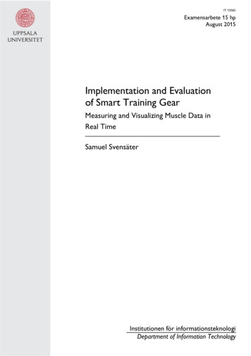
Figure 2: Forward rates, Zero rates and Swap rates curve of the data given inFigure 24 of Appendix 5where N is the nominal, y is the yield-to-maturity and C is the amount of thecoupon (C cN ). The present value of a bond is described by the followingequation: P V (y, f ) 1 yf T f N Cy 1 yf M 1with f equal to the frequency of the payment per year and M being the numberof remaining cash flows and T the time to maturity.There exist many different kinds of bonds like callable/putable (options onbonds), convertible (issued by companies, can be converted into stock), bulletbonds, etc. However, as most of interest rates derivatives can be seen as a seriesof Zero-Coupons bond, Swaps among them, in this dissertation we will focus onthe study of this kind of bonds.A Zero-Coupon bond is a bond that has just one single payment at maturitymade out of the principal plus (or minus) the interest rates, none intermediate coupons will happen. They are of great importance as they can be usedto discount and price interest rates derivatives. The idea under Zero-Couponpricing is taking all individual cash flows as if they where Zero-Coupon bonds.The evaluation of these cash flows is made using a yield curve or the discountfunction. This way of valuing interest rates derivatives is very popular especiallywhen pricing OTC (Over The Counter) instruments. In Figure 3 we can seehow a bond with several coupons can be seen as a sum of Zero-Coupon bonds.Furthermore, another important interest rates instruments are notes. A7
Figure 3: Bond scheme with several coupons vs Zero-Coupon bondsnote is similar to a bond with the difference that it has a shorter lifetime. Noteslifetime is usually between one and ten years, while bonds life is normally longer.Within notes, we can find the so-called Floating Rate Notes. The FRN are avery used financial instrument. They are quoted as a percentage of a notional,like bonds, however, FRN have reset dates. Every coupon date, the rate is resetin line with a money market reference, typically LIBOR, plus a fixed spread.The credit quality of the issuer is of great importance when pricing FRN, sinceif we wanted to trade it in the secondary market, the fixed spread should beshifted in case the rating of the issuer drops. Thus, when discounting, we haveto keep in mind the issuer discount curve p(0, i), where i is the current time.P NX[L(i 1, i) S]p(0, i) p(0, N )i 1will be the price of an FRN, where we discount the sum of LIBOR L(i 1) atthe previous coupon payment plus the spread S by the issuer discount to nextcoupon date i. We can estimate p(0, i) by the following formula:p(0, i) p(0, i 1)1 L(i 1, i) Q8
where Q is a measure of the credit quality of the issuer known as par floaterspread which changes over time. For the case where Q S we have that theFRN is traded at par. The spread over the LIBOR paid in order to make theFRN price at par is known as Discount Margin or Effective LIBOR spread andis calculated by iterations looking for the value of M in:(Lnext S) p PNi 11L S (1 L M )i(1 L M )N1 L Mwhere p is the bond price, L is the stub LIBOR coupon to next coupon date,Lnext is the next LIBOR payment and M is the discount margin which valuewe are looking for.The last instruments we will study in this section are the Forward RateAgreements. FRA are interest rate derivatives starting in the future withoutexchanging the principal. Thus, just differences on interest rates are tradedwhen the instrument matures. They are an agreement to borrow (or lend) anotional for a period of time at an agreed interest rate. This interest rate canbe lower or higher than the market rate set by the contract and so, it can beused to hedge or speculate. For example, if the rate of the FRA is set at 5% in6 months on LIBOR for 3 months and LIBOR stays at a lower level, lets say4%, the issuer of the FRA must pay the difference to the buyer for a 3 monthsperiod. They are very similar to Swaps (presented in Section 2.2) with thecontrast that FRA pay the difference of interest rates only once, at maturity.The value of an FRA is calculated as:P NτL(t, T ) K1 τ L(t, T )where t and T are start of the FRA and maturity respectively, K is the striketo be paid at t2 , and τ T t in days (taking a year as 360 days). FRA atpar (K L) are standardized nowadays because of its importance and are setas three month contracts between the famous IMM-days (third Wednesday ofMarch, June, September and December).2.2SwapsSwaps are among the most popular financial products that can be found inthe market nowadays and are the most traded ones by far when talking aboutfixed-income derivatives. A Swap is an agreement by which two counter-partiesexchange financial instruments periodically, mainly cash flows on a notional. Inthis case, one party agrees to pay the other party a cash flow equal to a fix rateon the notional and the other party pays floating rates cash flows (usually basedon an interest rate index like LIBOR or EURIBOR) on the same notional inexchange. It is easy to see how one can use it either to cover against possiblefluctuations on interest rates or to speculate under the idea of predicting thesefluctuations. Generally these agreements are taken by companies or financialinstitutions with the idea of hedging possible losses from rates.9
The present value of a Swap can be easily calculated discounting the payments and since commonly the notional is the same for both counter-parties, itwill not be exchanged. These payments will be done periodically at previouslydetermined dates called reset dates (monthly, every semester, annually, etc). Tobe able to price them, we have to calculate both the discounted fixed paymentsand the floating ones. However, as we can not determine the floating paymentsat the start of the contract, we have to estimate them calculating the forwardrate for each respective payment date of
Swaptions pricing under the single factor Hull-White Model through the Analytical formula and Finite Di erence Methods Victor Lopez Lopez1 Jan R oman2 1Corresponding author, student of the Master of Science in Mathematics with focus in Financial Engineering at Malardalen University.