WIXLIB

where K is a dimensionless constant in the range of 0 6 K 6 2, dependingon the amount of sunlight reflected by the satellite. R̂SA S is a vectorfrom the satellite to the sun, A is the cross sectional area of the satelliteperpendicular to R̂SA S and P is the momentum flux from the sun givenby P 4.4 · 10 6 [kg/ms2 ].The disturbance torque in SBRF is given byNR FR RCOM(11)where RCOM is a vector from the center of mass to the geometrical centerof the satellite.[1, Chapter 2.3.4]2.3Modelling EclipseThe satellite is only affected by solar radiation torques when the satelliteilluminated by the sun. Determining if the satellite is in eclipse can be doneby comparing the angles Θ and Ψ.!RLΘ arcsin(12)Rs/cRs/c is a vector from the center of the Earth to the satellite and RL is theradius of the Earth. Ψ arccos R̂L J · R̂s/c(13)RL J is a vector from the center of the Earth to the center of the sun.The satellite is in eclipse if Ψ 6 θ . [2, Ch 3.5]2.4Orbit PropagatorFor modeling of the position and velocity of the satellite, an orbit propagatormust be used. A Kepler orbit model is used here, not taking into accounteffects of Earth’s oblateness or the satellite drag.2.5Magnetic field modelIn order to simulate the behavior of magnetometers and magnetotorquers amodel of Earth’s magnetic field is needed. Here MATLAB’s built in functionwrldmagm from the Aerospace Toolbox is used. The function is based onthe World Magnetic Model for 2015-2020 from NOAA (North Oceanic andAtmospheric Administration) [3].10

2.62.6.1Attitude TransformationsDirection Cosine MatrixThe attitude of a three-dimensional body is conveniently described with aset of axes fixed to the body. The basic three-axis attitude transformationis based on the direction cosine matrix (DCM). Here, the 3-2-1, or ψ-θ-φ,Euler angle rotation sequence is used, which gives the following directioncosine matrix [4]. cθcψ [A321 ] cφsψ sφsθcψsφsψ cφsθcψ2.6.2 sθcθsψcφcψ sφsθsψ sφcθ (14) sφcψ cφsθsψ cφcθQuaternionsThe quaternion is a number system that extends the real numbers intoa four-dimensional domain similarly as the complex numbers extends thereal numbers into a two-dimensional domain. Quaternions can be used todescribe rotations of coordinate systems, and they provide a singularity-freerepresentation of kinematics. The quaternion is defined in the following wayq q4 îq1 ĵq2 îq3(15)where q1 ,q2 ,q3 and q4 are real numbers and î,ĵ and k̂ are unit vectors. Theseunit vectors satisfy the following conditions [4].î2 ĵ2 k̂2 1îĵ ĵî k̂ĵk̂ k̂ĵ îk̂î îk̂ ĵ2.6.3(16)The DCM and quaternionsThe DCM can be expressed in quaternions, 2q1 q22 q32 q422(q1 q2 q3 q4 ) q12 q22 q32 q42Aq 2(q1 q2 q3 q4 )2(q1 q3 q2 q4 )2(q2 q3 q1 q4 )If the DCM is expressed as112(q1 q3 q2 q4 ) 2(q2 q3 q1 q4 ) (17) q12 q22 q32 q42

Arw a11 a12 a13 a21 a22 a23 a31 a32 a33(18)the quaternions can also be found from from the elements of the DCM. q4 1 a11 a22 a33q1 0.25(a23 a32 )/q4(19)q2 0.25(a31 a13 )/q4q3 0.25(a12 a21 )/q4When q4 is very small, numerical inaccuracies may occur when calculatingthe remaining components. This problem can be solved by adding threeother equation sets, and always using the set for which the divisor componentis maximal. All of the equation sets are mathematically equivalent [4]. q1 1 a11 a22 a33q2 0.25(a12 a21 )/q4(20)q3 0.25(a13 a31 )/q4q4 0.25(a23 a32 )/q4 q3 1 a11 a22 a33q1 0.25(a13 a31 )/q4(21)q2 0.25(a23 a32 )/q4q4 0.25(a12 a21 )/q4 q2 1 a11 a22 a33q1 0.25(a12 a21 )/q4(22)q3 0.25(a23 a32 )/q4q4 0.25(a31 a13 )/q42.72.7.1Dynamics & KinematicsMagnetic actuationWhen using magnetic actuation, such as magnetotorquers, the attitude dynamics of the satellite can be described as Jω̇ ω Jω Tcoils Text(23)where ω is the angular rate of the satellite, expressed in SBRF. J is thetotal inertia matrix of the spacecraft, Tcoils is the vector of magnetic torquesproduced by magnetotorquers and Text is the vector of disturbance torques[2]. The magnetic moment of the magnetotorquers can be described asmmt nIA12(24)

where n is the number windings in the coil, I is the current and A areaenclosed by the magnetotorquers.The attitude kinematics is described by 1q̇ Ω ω q2(25) where Ω ω is a 4x4 skew symmetric matrix defined in below: 0ω3 ω2 ω1 ω30ω1 ω2 , ω R3Ω ω ω2 ω10ω3 ω1 ω2 ω3 02.7.2(26)Reaction Wheel actuationThe attitude dynamics, of a satellite with reaction wheels, can be modeledasω̇ J 1 (ω Jω) J 1 (ω h) J 1 Tw J 1 Te(27)where Jis the total inertia matrix of the spacecraft, now also including thereaction wheels, h is the angular momentum of the reaction wheels, Twis the torque produced by the reaction wheels acceleration and Text is theexternal disturbance torque. The angular momentum of the reaction wheelsis given below [5].ḣ Tw(28)13

3DetumblingWhen a satellite separates from it’s launcher, it tumbles in space in an uncontrolled manner. Before the satellite can begin its nominal operation, theangular velocity has to be reduced. The purpose of the detumbling controller is to dampen the angular velocity vector of the satellite. A satellitein LEO with an altitude of 400 km is considered detumbled when its angularrate has decreased to 0.13 /s or less [1].To test the detumbling algorithm, a modeling environment is to be set upin MATLAB. The algorithm is to be written in C, and with some modifications they shall be able to be executed on ÅAC’s target environment OBC.There exists a number of different detumbling controllers and some of themare tested in [6] for a 2U CubeSat. Controllers based on magnetometerfeedback, gyroscope feedback, sun sensor feedback and passive control arecompared in terms of maneuver time, precision, control effort, robustnessand implementation. The magnetometer feedback B-dot controller was concluded to be the best and easiest controller to implement for a 2U CubeSat.The B-dot controller is chosen in this project because it is the easiest andmost common detumbling controller for small satellites.3.1The B-dot ControllerThe torque produced by magnetic torquers is given byL m B(29)where m is the commanded magnetic dipole moment generated by the torquers and B is the local geomagnetic field expressed in body-frame coordinates. Detumbling from arbitrary initial spinning of the satellite is accomplished by commanding the magnetic dipole moment of the magnetometersbykm Ḃ(30)kBkwhere K is a positive scalar gain [7]3.2Design SpecificationA simulation framework in MATLAB, with the structure of the block diagram in Fig.2, shall be built. This framework shall include an orbital propagator, an attitude propagator, a function to calculate attitude disturbancetorques and a function that acts as a magnetometer. Orbital, satellite andhardware parameters (such as magnetotorquer size) shall be easy to change.The control loop is written in C and it shall:14

get the magnetometer readings (from the simulation of magnetometersin the MATLAB workspace) calculate the control torque needed to detumble calculate the magnetotorquer current needed to detumble set the magnetotorquer current (put the current values into the MATLAB simulation workspace)The control loop is a C-source function that shall be called from the mainprogram in MATLAB. Therefore the control loop file must also contain agateway function (mexFunction) between C and MATLAB. The control loopfunction can the be called like a regular MATLAB function from the MATLAB workspace. The four C-functions run by the control loop are regularC-source functions. (For more information on MEX-files, see the MATLAB documentation on MEX-files.)All MATLAB variables are by default double-precision floating point variables and stored as mxArrays. The mxArray is the fundamental MATLABtype in C. Though MATLAB supports single-precision floating-point and8-, 16-, 32-, and 64-bit integers, both signed and unsigned.15

Figure 2: A block diagram of the structure of the simulation frameworktogether with the detumbling controller.3.3Module specificationsHere, the function of all the modules from the block diagram in Fig. 2 aredescribed and the input and output parameters of every block are shown.main.mSimulation main program: MATLAB script to run the simulation, the scriptshould also plot the position, attitude, velocity, angular rate, control anddisturbance torques.set int param.mMATLAB-function where the integration parameters for the simulation aredefined and set. The parameters can easily be changed inside the functionbefore running the simulation.The function takes no input and the output is the following parameters:16

set int param.mIN/OUT NameOUTdtOUTt0OUTtfOUTtimeDescriptionSimulation time step [s]Simulation start time [s]Simulation end time [s]Simulation time vector [s]TypedoubledoubledoubledoubleTable 1: IN/OUT parameters of set int param.mset sat param.mMATLAB-function where the satellite properties, orbital parameters andthe hardware parameters are defined and set. The parameters can easilybe changed inside the function before running the simulation. The functiontakes no input and the output is the following parameters:set sat param.mIN/OUT NameSatellite TSAT.QUATERNIONOUTSAT.ANGULAR RATEOUTSAT.COMOUTSAT.COPOUTSAT.GEO CENTROUTSAT.CIRC ESTOrbital .SEMI MAJOR AXISOUTSAT.INCLINATIONOUTSAT.RIGHT ASCENSION 0OUTSAT.ARGUMENT OF PERIGEE 0OUTSAT.MEAN ANOMALYMagnetotorquer parametersOUTSAT.MAGNETOTORQUER AREAOUTSAT.MAGNETOTORQUER NOUTSAT.RATE HIGH LIMITDescriptionTypeTotal satellite mass [kg]Satellite side length [m]Satellite inertia [kg*mˆ2 ]Initial attitude [quaternions]Initial angular rate [rad/s]Satellite Center of Mass [m]Satellite Center of Pressure [m]Satellite geometrical center [m]Radius of estimated spherical satellite edouble[rad][km][km][rad]Initial argument of right ascension [rad]Initial argument of perigee le[mˆ2]Number of turns of magnetotorquer coilAngular rate limit for detumbling [rad/s]doubledoubledoubleTable 2: IN/OUT parameters of set sat param.msat pos vel.mMATLAB-function to compute current satellite position and velocity in ECIcoordinate system. The IN/OUT parameters are described in table 3.17

sat pos vel.mIN/OUT NameINSATINOUTOUTtimepos satvel satDescriptionArray containingall satellite parameters.Current time [s]Satellite position in ECI [km]Satellite velocity in ECI [km]TypedoubledoubledoubledoubleTable 3: IN/OUT parameters of sat pos vel.mcalc dcm.mMATLAB-function to calculate the direction cosine matrix for coordinatesystem transformations from ECI to SBRF reference frame.calc dcm.mIN/OUT NameINquaternionOUTdcmDescriptionAttitude quaternion vectorDirection cosine matrixTypedoubledoubleTable 4: IN/OUT parameters of calc dcm.mcalc env torque.mMATLAB-function to calculate environmental disturbance torque affectingthe satellite: torque produced by aerodynamic drag, torque produced by thegravitational gradient and torque produced by solar radiation. For calculating torque generated by atmospheric drag, a built in MATLAB function(atmosnrlmsise00 from MATLAB Aerospace Toolbox) for calculating theatmospheric pressure will be used here. The IN/OUT parameters are described in the table below.18

calc env tor.mIN/OUT NameINSATINININOUTOUTOUTOUTpos satvel satdcmtot env torquesn aero sbrfn gg sbrfn solar sbrfDescriptionArray containingall satellite parameters.Satellite position in ECI [km]Satellite velocity in ECI [km]Direction Cosine MatrixTotal environmental torques [Nm]Torque produced by aerodynamic drag [Nm]Torque produced by gravity gradient [Nm]Torque produced by solar radiation [Nm]Table 5: IN/OUT parameters of calc env torque.mcalc magn.mMATLAB-function to calculate the magnetic field strength. A MATLABbuilt-in function ,wrldmagm from MATLAB Aerospace Toolbox, for calculating the magnetic field strength will be used here. The values fromwrldmagm are given in the north east down coordinate system so they haveto be converted into the SBRF. The IN/OUT parameters are described inthe table below.calc magn.mIN/OUT NameINSATININOUTOUTOUTpos satdcmb sbrf xb sbrf yn gg sbrfDescriptionArray containingall satellite parameters.Satellite position in ECI [km]Direction Cosine MatrixMagnetic field in the x-direction [T]Magnetic field in the y-direction [T]Magnetic field in the z-direction [T]TypedoubledoubledoublefloatfloatfloatTable 6: IN/OUT parameters of calc magn .mcontrol loop.cC-function, this is the control loop which shall run the following four Cfunctions. This function shall run once at every time step of the simulation.This function should also include a mexFunction, a gateway function fromC to MATLAB. The IN/OUT parameters are described in table double

control loop.cIN/OUT NameINdtINgainINnumber of turnsINmt areaDescriptionTimestep between magnetometer readings [s]Controller gainNumber of turns of magnetotorquer coilMagnetotorquer area [mˆ2]Table 7: IN/OUT parameters of control loop.cget magn values.cC-function to get readings from the magnetometer (magnetometer readingsfrom MATLAB simulation workspace), and save these values until the nextiteration of control loop. The IN/OUT parameters are described in table 8.get lues.cNametimemagn value xmagn value ymagn value zlast value xlast value ylast value zDescriptionCurrent time [s]Magnetic field strengthMagnetic field strengthMagnetic field strengthMagnetic field strengthMagnetic field strengthMagnetic field strength[T][T][T][T][T][T]Typeuint32 tfloatfloatfloatfloatfloatfloatTable 8: IN/OUT parameters of get magn values.ccalc contr torque.cC-function to calculate the control torque needed to detumble the satellite using the B-dot detumbling algorithm. The IN/OUT parameters aredescribed in table 9.20Typefloatfloatfloatfloat

calc contr torque.cIN/OUT mag field xmag filed ymag filed zlast mag field xlast mag field ylast mag field zcontr tor xcontr tor ycontr tor zDescriptionTimestep betweenmagnetometer readings [s]Detumble controller gainMagnetic field strength [T]Magnetic field strength [T]Magnetic field strength [T]Magnetic field strength [T]Magnetic field strength [T]Magnetic field strength [T]Control torque [Nm]Control torque [Nm]Control torque oatfloatfloatTable 9: IN/OUT parameters of calc contr torque.cconvert torque to current.cC-function to calculate magnetotorquer current needed to detumble thesatellite. The IN/OUT parameters are described in table 10.convert torque to current.cIN/OUT NameINcontr torque xINcontr torque yINcontr torque zINn of turnsININ/OUTIN/OUTIN/OUTmt areacurrent mmt xcurrent mmt ycurrent mmt zDescriptionControl torque [Nm]Control torque [Nm]Control torque [Nm]Number of turns ofmagnetotorquer coilMagnetotorquer area [mˆ2]Magnetotorquer current [A]Magnetotorquer current [A]Magnetotorquer current le 10: IN/OUT parameters of convert torque to current.cset current.cC-function to set the magnetotorquer current, here putting the current values into the MATLAB simulation workspace. Because the MATLAB standard type is double, it is easiest to send double parameters to MATLAB.The IN/OUT parameters are described in table 11.21

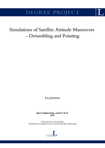
set current.cIN/OUT NameIN/OUT currentIN/OUT currentIN/OUT currentOUTcurrentOUTcurrentOUTcurrentmmt xmmt ymmt e 11: IN/OUT parameters of set current.cattitude dynamics.mMATLAB-function to calculate the attitude and the angular velocity of thesatellite, taking environmental disturbances and control torques into account. The IN/OUT parameters are described in table 12.attitude dynamics.mIN/OUT NameINtimeINxINININOUTcontrol torqueenv torqueinertiadxDescriptionCurrent time [s]Angular rate [rad/s] and attitude(quaternions)Control torque vector [Nm]Environmental torque vector [Nm]Inertia of satellite [kg*mˆ2]Change of attitude and angular ble 12: The IN/OUT parameters of attitude dynamics.m3.4Simulation ResultsThe b-dot control law in Eq. (29) was simulated for a small satellite in lowearth orbit, the altitude of the orbit is 400 km and the inclination is 45 . Theinitial angular rate is set to ω0 [ 5.7 5.7 5.7 ] deg/s. The controller gain isset to k 1.5 103 . The angular velocities are shown in Fig. 3, and a zoomof the angular velocities in Fig. 4 shows that the controller has detumbledthe satellite to 0.13 /s in 5500 s (92 min). Thus the controller manages todetumble the satellite in about one orbit. The associated magnetic controltorques are shown in 5.22

Figure 3: The angular rate for the detumbling simulation of the control lawin Eq.(29).Figure 4: A zoom of the angular rate for the Detumbling simulation of thecontrol law in Eq.(29)).23

Figure 5: Control torques for the Detumbling simulation of the control lawin Eq.(29).24

4Pointing4.1Literature ReviewResearch in attitude maneuvers has been carried out since the beginning ofspace missions. Emphasis has been put on the development of time-optimalmaneuvering methods for spacecraft and robust control schemes to accountfor disturbances.The aim of this text is to review time-efficient attitude maneuverer availabletoday and compare these algorithms to the closed-loop quaternion feedbackalgorithm. The main focus is put on a rigid spacecraft without appendages,using reaction wheels as actuators. Two to three of these algorithms willbe chosen for simulation in MATLAB to examine their performance. Thesealgorithms will be reviewed in terms of: Maneuver time Robustness (ability to handle unexpected disturbances) Stability Applicability for implementation on an on-board computerTo put the current algorithms in context, a small overview of earlier advancements within the field of time-optimal control will first be presented.Then a current time-optimal algorithm suitable for attitude control will bepresented. Because the time-optimal algorithm is not executable in realtime, it is of interest to bring up other algorithms that are not necessarilytime-optimal but time-efficient and executable in real time.4.1.1BackgroundIn a survey of time-optimal attitude maneuvers [8] the literature coveringthe advancements within time-optimal control, from the sixties until theyear of publication 1994, is reviewed. A closed-loop control for a rest-torest Louvre and a tracking maneuver is presented in [9]. In this paper, th

2.3 Modelling Eclipse The satellite is only a ected by solar radiation torques when the satellite illuminated by the sun. Determining if the satellite is in eclipse can be done by comparing the angles and . arcsin RL R s c! (12) R s c is a vector from the center of the Earth to the satellite and RL is the radius of the Earth. arccos R L! J R !