WIXLIB

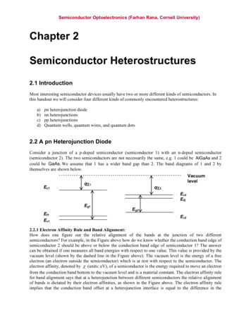
Semiconductor Optoelectronics (Farhan Rana, Cornell University)emission term in Equation (4) and determine carrier density from Equation (5) and once the carrierdensity has been determined using Equation (5) for a given current bias, the photon density can bedetermined using Equation (3).11.5.4 Regime III ( n nth ) – Laser near Threshold:As the current is increased further, at some current value the carrier density, as predicted by Equation (5),will equal the threshold carrier density n th . The current for which the carrier density, as predicted byEquation (5), equals the threshold carrier density is called the threshold current and is given as, i Ith Rnr nth Gnr nth Rr nth Gr nth (6)qVaWhen the carrier density n equals the threshold carrier density n , the gain g equals the threshold gainthg th and the photon density, as given by Equation (3) is infinite because the denominator is zero. In fact,if the carrier density were to exceed the threshold carrier density, the photon density, as given byEquation (3), would be negative – an obviously unphysical result. What is happening is that as the currentis increased, and the carrier density increases and approaches the threshold carrier density, the gainapproaches the threshold gain. As the gain increases, the simulated emission rate increases andapproaches the rate at which the photons are lost from the cavity. Every photon in the cavity now has achance to multiply before it is lost from the cavity and so the steady state photon population inside thecavity also increases. Equation (3), reproduced below,nsp av g g Vpnp 1 av g g ppredicts that as the gain g approaches the threshold gain g , and optical gain v g approaches thetha goptical loss 1 p , the steady state photon density increases significantly because the denominatorapproaches zero. When the photon density becomes very large, Equation (5) is no longer valid becausecarrier recombination rate due to the stimulated emission cannot be ignored compared to the other nonradiative and radiative recombination rates. Therefore, Equation (4) has to be used to calculate the carrierdensity in steady state. Equation (4) shows that as the photon density increases significantly, thestimulated emission rate av g g n p also increases and keeps the carrier density, and therefore the gain,from increasing as much with current as when the stimulated emission rate is ignored. In fact, because thephoton density increases drastically when the optical gain av g g gets close to the optical loss 1 p , theincreased stimulated emission rate never allows the carrier density to ever exceed the threshold carrierdensity nth and, therefore, the gain never exceeds the threshold gain g th . This gain saturation broughtabout by a large photon density is needed to stabilize the photon density inside the cavity. If the opticalgain were to exceed the threshold gain then the photon multiplication rate due to stimulated emissionwould exceed the photon loss rate and the steady state photon density would increase to infinity. In otherwords, there would be no steady state and this is the reason why Equation (3) predicts a negative photondensity for av g g 1 p .The Figure below shows the carrier density and the photon density vs. the current for regimes I-III.

Semiconductor Optoelectronics (Farhan Rana, Cornell University)nnpnthntrIIthIthI11.5.5 Regime IV ( n nth ) – Laser above Threshold:When the current is increased beyond the threshold current Ith , the photon density becomes so large thatthe resulting increased recombination due to stimulated emission prevents the carrier density fromincreasing beyond nth . The carrier density gets fixed at a value close to (but less than) nth . To find thephoton density when I Ith , we start from Equation (4) and subtract Equation (6) to get, i I Ith qVa Rnr n Gnr n Rr n Gr n Rnr nth Gnr nth Rr nth Gr nth v g g npSince for I Ith , n nth and g g th 1 av g p , the term inside the curly brackets is close to zero,and we get, i I Ith qVa np a p Np npVp i I Ith pqThe above equation shows that the photon density increases linearly with the current when the currentexceeds the threshold current. The point where I Ith is called the “threshold for lasing” or just as the“laser threshold.” Above threshold, the carrier density n , and the optical gain g , remain fixed to theirvalues at threshold, and the photon density increases with the current and the corresponding increase inthe stimulated emission rate is just enough in order to maintain the carrier density at its threshold value asthe current is increased. The Figure below shows the carrier density and the photon density vs. the currentfor a laser operating below and above threshold. The rapid buildup of photon population when I Ith iscalled lasing.nnpnthntrIthIIthI

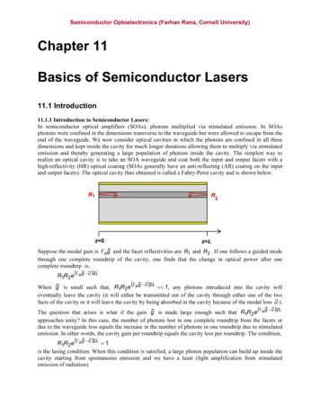
Semiconductor Optoelectronics (Farhan Rana, Cornell University)11.5.6 Laser Output Power above Threshold:The output power of the laser is the power coming out from the two end facets of the laser cavity. Since,Npn pVpP o o p pthe laser power above threshold in terms of the current is,Np I Ith P o o i pqThe above expressions shows that if o i were equal to unity then every electron injected into the laserper second above the threshold injection rate of Ith q would end up producing a photon in the laseroutput. Above threshold, the laser is therefore a very efficient converter of electrical energy into opticalenergy. This property of the laser is commonly expressed in terms of the differential slope efficiency dS ,dP dS o idIqor the differential quantum efficiency dQ , dQ q dP o i dI11.5.7 A Worked Example:Consider an InGaAsP/InP laser (shown in the Figure below) with the following parameter values:Insulator1.5 mOptical Power (mW)Top metalInP substrateCurrent (mA)(LEFT) Output facet of a 5 QW InGaAsP/InP laser for 1.55 m operation. (RIGHT) Measured LIcharacteristics of the laser.A multiple quantum well (MQW) activeregion with 7 nm wells, 9 nm barriersand 100 nm SCH regions.Laser length L 500 mp dopedSCHSCHn doped

Semiconductor Optoelectronics (Farhan Rana, Cornell University)Active region width W 1.5 mActive region height (all 5 quantum wells) h 0.035 m 35 nmFacet reflectivities R1 R2 0.3Transparency carrier density ntr 1.75x1018 1/cm3Active region mode confinement factor (for all 5 quantum wells) a 0.07Waveguide group velocity vg c/3.4Waveguide modal loss 15 1/cmA 0B 10-9 cm3/sC 5x10-29 cm6/sg o 1500 1/cmCurrent injection efficiency i 0.85Using the above parameters we can calculate the remaining laser parameters as follows. The effectivemirror loss is,1 1 m log 24 1/cmL R1R2 The output coupling efficiency is, o m 0.62 mThe photon lifetime in the cavity is, vg11 v g m log RRL p1 2 p 2.9 ps v g The threshold gain is,1 v g a g th p g th 558 1/cmSince, n g g o log ntr we can calculate the threshold carrier density, nth n tr e gth go 2.59 1018 1/cm3From the threshold carrier density we can obtain the threshold current, i I th23 R nr nth Gnr nth R r nth Gr nth Anth Bnth CnthqVa I th 37.5 mAThe calculated threshold current value compares favorably with the observed value in the Figure above.

Semiconductor Optoelectronics (Farhan Rana, Cornell University)11.6 Laser Stability and Relaxation Oscillations11.6.1 Introduction:Suppose a laser is biased with current I above threshold. The steady state values of carrier and photondensities are n and n p , respectively. Since I I th , n n th . Suppose at time t 0 , the carrier density issuddenly increased from n to n n . The new value of the carrier density is not the steady state valueand we would like to see how, if at all, the steady state value is recovered. The carrier density n n isgreater than n th , and, consequently, the gain g is greater than the threshold gain g th . In steady state, g can never be greater than g th , but this restriction does not hold in non-steady state situations.Alternatively, we could have perturbed the photon density at time t 0 to n p n p . If the carrier orphoton densities in a laser are disturbed (by some means) from their steady state values then it isimportant to know if these quantities return to their steady state values. If they do, the laser is stable. Ifthey don’t, the laser is unstable. Studying the recovery dynamics associated with such carrier density orphoton density perturbations tell a lot about the underlying laser physics.We start from the laser rate equations,dn i I Rnr n Gnr n Rr n Gr n v g g npdt qVa 1 n sp a v g g n p a v g gdt p Vp and make the substitutions,n n n t n p n p n p t dn pThe laser rate equations contain many nonlinear terms and we will linearize each of these terms aroundtheir steady state values and keep terms to only first order in the perturbed quantities, n t and n p t .This procedure yields,dg v g g n p v g g n p vgn p n t v g g n p t ssdn ss n t n p t v g g n p ss st a p Rnr n Gnr n Rr n Gr n Rnr n Gnr n Rr n Gr n ss d Rnr n Gnr n Rr n Gr n n t dnss n t Rnr n Gnr n Rr n Gr n ss av g g n p a v g g n pss av gdg n p n t av g g n p t dn ss n t n p t av g g n p a ss st p r

Semiconductor Optoelectronics (Farhan Rana, Cornell University)We have introduced two new quantities in the above equations; the differential stimulated emission time st and the differential recombination time r , defined as follows,1d Rnr n Gnr n Rr n Gr n r dnss 1dg vgnpdn ss st The laser rate equations result in the following linear coupled differential equations for the perturbations, I1 I d n t r st a p n t n p t adt n p t 0 st We have ignored the perturbation in the spontaneous emission term in the laser rate equations since it ismuch smaller than the perturbation in the stimulated emission term.11.6.2 Relaxation Oscillations:The coupled differential equations for the perturbations in the carrier and photons densities constitute asecond order linear system much like the equations for the current and the voltage in a LCR circuit. Thecoupled equations give the following identical second order differential equations for the perturbations,d 2 n p t dt2d n t d n p t dt2 R n p t 0d n t 2 R n t 0dtdtwhere the relaxation oscillation frequency R and the damping constant are defined as,dg n p1 R vgdn ss p st p22 I r I stThe solutions of the above second order equations have the form, 2 2 t 2 2 n t e 2 A cos R t B sin R t 2 2 2 2 2 n p t t D sin R t 2 2 The constants A, B, C, and D can be chosen to satisfy the initial conditions. Suppose, n p t 0 0then we get, t 2eC cos R2

Semiconductor Optoelectronics (Farhan Rana, Cornell University)A n t 0 n t 0 B 2C 0D R2 a n t 0 2 22 st 2 The Figure below shows the time evolution of the carrier density and photon density perturbationsvertical scale is normalized). The perturbations are damped and the steady state is stable because anydisturbances or perturbations decay with time. The decay is not monotonic but involves damped carrierand photon density oscillations that are 90-degrees out of phase. These oscillations are called relaxationoscillations. If the second order system is critically damped or over damped (i.e., R 2 ) then theperturbations will decay monotonically without any relaxation oscillations. R2 np(t)t n(t)11.7 Direct Current Modulation of Lasers11.7.1 Introduction:Consider the LI (light vs. current) curve of a semiconductor laser. Suppose the laser is biased with currentI and the corresponding output power is P .PowerPINow suppose the current is varied such that,I t I I t thICurrent

Semiconductor Optoelectronics (Farhan Rana, Cornell University)The output power can be written as,P t P P t This current modulation is used in optical communication systems to transfer information from theelectrical domain to the optical domain. The question we need to answer here is how fast can a laser bemodulated? The answer can be obtained from the laser rate equations. We assume that,n t n n t n p t n p n p t As in the previous Section, we linearize the laser rate equations and obtain, II 1 d n t r st a p n t i I t 1 n p t aqVa 0 dt n p t 0 st We assume that the time varying part of the current, carrier density, the photon density, and the outputpower are sinusoidal,I t I Re I f e i 2 ft n t n Re n f e i 2 ft n p t n p Re n p f e i 2 ft P t P Re P f e i 2 ftThe solution is, i 2 f n f I f 2 H f n f iqVa R p a p The solution above relates the small signal carrier and photon densities to the small signal current. Thechange in the output power is, P f o iH f I f qThe modulation response function H f is,H f R22R 2 f 2 i 2 f Note that since H f 0 1 , P f 0 o i I f 0 qThis low frequency result could also have be obtained directly from the relation, P o i I I th qAlso note that, n f 0 0 . This result is to be expected since the carrier density in steady state abovethreshold does not vary with current, and remains fixed at a value close to n th .11.7.2 High Frequency Response of Lasers:The relation,

Semiconductor Optoelectronics (Farhan Rana, Cornell University) H f I f qshows that the frequency response of the laser power to current modulation is governed by the functionH f . In optical communication systems, a detector at the receiving end converts the modulated lightback into current. A schematic of a communication link is shown in the Figure below. Assuming thefrequency dependent detector responsivity to be R f , the RF current at the output of the link is related tothe RF current at the input to the link by the relation, Iout f R f P f R f o iH f I in f qThe ratio of the RF power at the output to the RF power at the input is called the link loss and itsexpression is (assuming no optical losses in the fiber and no coupling losses), P f o i Iout f I in f 22 R f o i H f q2The ratio is proportional to H f .2 Iout(f) Iin(f) P(f)LoadILaserFiberVDetectorAn optical communication link using a directcurrent modulated semiconductor laser10110110 H(f) 2 H(f) 2Increasingcurrent0-110 -21010-102 f/ RThe Figure above plots H f 210101100-110 -210-1100102 f (rad/s)as a function of frequency. The peak of H f 2101102occurs at a frequency fequal to approximately R 2 (provided R ). The peak is called the relaxation oscillation peak.The frequency f3dB at which H f decreases from its value at zero frequency by 3 dB (by a factor of 2)2is approximately equal to 1 2 R 2 (provided R ). f3dB is the maximum frequency atwhich the laser power can be current modulated. The relaxation oscillation frequency R 2 therefore

Semiconductor Optoelectronics (Farhan Rana, Cornell University)sets the scale for the maximum frequency at which a laser can be current modulated. The relaxationoscillation frequency, given by the expression,1dg n p vg R dn ss p st pincreases as the square-root of the steady state photon density. Therefore, increasing the current willincrease the frequency f3dB . However, this trend does not continue to very high current levels. This isbecause the damping constant, given by,IIIdg vgnp dn ss r st rincreases linearly with the photon density (faster than the relaxation oscillation frequency). When thelaser current is slightly larger than the threshold current, R because 1 p 1 st ,1 r . Whenthe current is increased, f3dB also increases. As the current is increased to larger values, at some point therelaxation oscillation frequency R becomes equal to oscillation peak in H f 2 . When this happens, the relaxation2disappears and f3dB equals R 2 2 2 p . If the current is increasedbeyond this point, the frequency f3dB decreases instead of increasing. The maximum value of f3dB istherefore related to the inverse photon lifetime in the cavity,f3dB max 22 pThe inverse photon lifetime sets the upper limit on the modulation speed of semiconductor lasers.11.8 Band Diagrams and Circuit Models11.8.1 Band Diagram:In a laser, one must have the following condition satisfied,E fe E fh qV E gThe band diagram is shown in the Figure below.EfeqVEfhIn the active region, the electron density n is a function of the Electron Fermi level, the hole density p isa function of the hole Fermi level and quasineutrality implies,n E fe p E fh The above relation, together with the condition, E fe E fh qV , uniquely determines the carrier densityin the active region as a function of the voltage V across the junction.

Semiconductor Optoelectronics (Farhan Rana, Cornell University)11.8.2 Electrical Impedance of the Active Region:Consider a laser operating in steady state. The impedance Z f of the active relates the small signalcircuit current I f to the small signal voltage V f across the junction, V f I f Z f A small change in the carrier density n f can be related to a small change in the voltage V f asfollows, n n f V f V ssThe laser rate equations in Section 11.7 give, i 2 f I f n f H f i2qVa RThe above three Equations give,11 V f i 2 fZ f H f i 2qVa n V ss I f RThe impedance of the active region is proportional to the modulation response function H f . At lowfrequencies, when H f 1, the impedance of the active region is inductive and approaches zero as thefrequency approaches zero.11.8.3 Total Electrical Impedance:Consider the laser connected as shown below. Th

R R e ag L is called the threshold gain gth . We can write the expression for the threshold gain as, 1 log 1 1 2 L R R agth The threshold gain is function of the parameters of the optical cavity. The lasing condition states that photons multiply via stimulated emission at the same rate inside the cavity as the rate at which they are