Transcription
Munich Personal RePEc ArchiveDoes Federal Crop Insurance MakeEnvironmental Externalities fromAgriculture Worse?Weber, Jeremy G. and Key, Nigel and O’Donoghue, ErikUniversity of Pittsburgh, Graduate School of Public andInternational Affairs, USDA Economic Research Service, USDAEconomic Research Service13 May 2016Online at https://mpra.ub.uni-muenchen.de/71293/MPRA Paper No. 71293, posted 15 May 2016 07:43 UTC
Does Federal Crop Insurance Make Environmental Externalities from Agriculture Worse?Jeremy G. Weber*, Nigel Key**, Erik O’Donoghue**FORTHCOMING IN THE JOURNAL OF THE ASSOCIATION OF ENVIRONMENTALAND RESOURCE ECONOMISTSAbstract: Farmers dramatically increased their use of federal crop insurance in the 2000s. From2000 to 2013, premium subsidies increased seven-fold and acres enrolled increased by 77percent. Although designed for non-environmental goals, subsidized insurance may affect theuse of land, fertilizer, and agrochemicals and therefore environmental externalities fromagriculture. Using a novel panel data, we examine farmer responses to changes in coverage withan empirical approach that exploits program limits on coverage that were more binding for somefarmers than for others. Estimates indicate that expanded coverage had little effect on the shareof farmland harvested, crop specialization, productivity, or fertilizer and chemical use. Morebroadly, we construct and describe a new nation-wide, farm-level panel data set with nearly32,500 farms observed at least twice over the 2000-2013 period, a resource that should enrichU.S. agro-environmental research.JEL Codes: Q15, Q18, Q12,Keywords: Crop insurance, agriculture, environmental externalities, fertilizer*Assistant Professor, University of Pittsburgh, Graduate School of Public and International Affairs andDepartment of Economics, 3601 Wesley W. Posvar Hall, Pittsburgh, Pennsylvania 15260, 412.648.2650,jgw99@pitt.edu.**Economists at the USDA Economic Research Service, nkey@ers.usda.gov andeodonoghue@ers.usda.gov.The views expressed are those of the authors and do not necessarily reflect the views or policesof the U.S. Department of Agriculture1
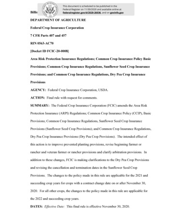
The decisions of crop farmers, such as how much fertilizer and pesticide to use, can affectbiodiversity and water quality. Hendricks et al. (2014), for example, find that increased demandfor corn-based ethanol expanded the so-called dead zone in the Gulf of Mexico by encouragingfarmers to plant more corn and use more fertilizer. U.S. federal crop insurance may have similarunintended effects. Although designed to reduce farm income variability, crop insurance maycause farmers to take more risks and apply more fertilizer, plant crops on erodible lands, orspecialize in fewer crops, thereby exacerbating environmental externalities from agriculture.The growth in federal crop insurance warrants greater study of the program’s unintendedconsequences (Goodwin and Smith, 2013). Crop insurance has expanded significantly since2000 and with the 2014 Farm Act is now the main conduit of financial support to farmers.Between 2000 and 2013, acres enrolled beyond the most basic coverage increased by 77 percent.The corresponding premium subsidies paid by the federal government also increased. Before2000 the subsidies never exceeded a billion dollars in real terms; for the years 2011-2013, theyranged between 6 and 7 billion annually (Figure 1).The empirical literature on crop insurance provides a generally weak foundation fordistinguishing the effect of insurance apart from confounding factors. There are no farm-levelempirical studies of crop insurance and input use that use a sample of national scope and controlfor farm fixed effects. Studies have commonly relied on cross-sectional variation (e.g. Horowitzand Lichtenberg, 1993; Smith and Goodwin, 1996), even though time-invariant unobservablevariables such as land quality and risk attitudes are likely correlated with crop insuranceparticipation and input use. O’Donoghue, Roberts, and Key (2009) is an exception, but it onlyconsiders crop diversification, not input use.2
Almost all published studies also assume that crop insurance participation is exogenousto farm decisions. This is unlikely. Farmers may shift land from low-input, non-insurable uses tohigh-input, insurable crops (or vice versa) for reasons unrelated to insurance such as changingcrop prices or farm finances. With the new land use eligible for subsidized insurance,participation in insurance would increase along with input use, inducing a spurious correlationbetween the two. Here, Cornaggia (2013) is a notable exception in his treatment of theendogeneity of insurance adoption. He exploits the introduction of new insurance policies insome counties and not others. However, his data only permit examining the effect of insuranceon yields, and his identification strategy rests on 14 insurance policy events, with all but oneoccurring before the beginning of our study period.We study how changes in insurance coverage over the 2000-2013 period affected farmlevel crop choice and fertilizer and chemical use while controlling for farm-fixed effects and theendogeneity of crop insurance participation. Controlling for farm-fixed effects is possible by ourcreation of a panel data set constructed from 14 years of the annual USDA Agricultural ResourceManagement Survey. For plausibly exogenous variation in coverage, we exploit the insuranceprogram’s limit on how much coverage farmers could purchase. As the incentive to haveinsurance grew, farmers who initially had little coverage could greatly expand coverage; farmersalready close to the maximum level could not. Instrumenting the change in coverage with eachfarm’s initial coverage ratio–its actual coverage relative to its farm-specific maximum coveragepossible‒allows us to identify the effect of coverage on production decisions under plausibleassumptions. Moreover, the non-linear relationship between the initial coverage ratio and thesubsequent change in coverage allows us to control (linearly) for the initial level of crop3
insurance coverage in our regressions, making our approach robust to a linear relationshipbetween initial coverage and changes in production decisions.In addition to providing plausible estimates of the effects of insurance coverage, wecreate and document a new farm-level panel data set that will enrich future research inagriculture and environmental policy. Empirical research related to U.S. farms has been limitedby the lack of nation-wide panel data at the farm level. Outside of the Census of Agriculture,which has a limited scope of questions and occurs once every five years, there has been nocomprehensive panel data for U.S. farms. Our panel data set is based on the AgriculturalResource Management Survey–the only annual nation-wide data source on the finances,production practices, and resource use of U.S. farms and the households operating them. Despiteits design as a cross-sectional survey, nearly 32,500 farms have been surveyed at least twice overthe 2000-2013 period, thereby providing a rich resource to study dynamic issues and account fortime-invariant farm heterogeneity.Applying the data to study the effects of crop insurance, our OLS estimates from a firstdifferenced model show a positive relationship between coverage and fertilizer and chemical use,though smaller than some prior estimates using cross-sectional data. Our instrumental variableestimates, however, show that coverage has little effect on crop specialization or input use. Theestimates are sufficiently precise that even the upper bounds of a 95 percent confidence intervalrepresent environmentally negligible effects. Thus, it does not appear that a more generous cropinsurance program by itself encourages specialization or greater fertilizer and chemical use asseveral prior studies have found.4
1 AGRICULTURE, THE ENVIRONMENT, AND CROP INSURANCE1.1 Agriculture and the EnvironmentFarmers are the chief managers of arable lands around the world, and their decisions affectenvironmental quality on their lands and beyond (Tilmen et al., 2002). Switching marginal landfrom passive uses into cultivation reduces its value as wildlife habitat. Marginal lands are alsomore prone to soil erosion when cultivated, leading to the sedimentation of lakes and streams(Shortle, Abler, and Ribaudo, 2001). For land already in cultivation, a less diverse crop mixreduces biodiversity and increases insect and disease problems (Sulc and Tracy, 2007; Landis,2008).Fertilizer nutrients or pesticides running into surface water or leaching into groundwatercan be extensive. The U.S. Environmental Protection Agency has identified agricultural nonpointsource pollution as a leading source of impairment of the country’s water resources (U.S. EPA,2015). Studies have shown that 30 to 40 percent of nitrogen fertilizer applied to crop fields seepsinto ground or surface water, with losses of 70 percent on the margin (Cambardella et al., 1999;Randall and Mulla, 2001; Li et al., 2006). A ten-year study by the U.S. Geological Survey foundwidespread occurrences of pesticides in streams and groundwater, often at concentrationsdeemed harmful to aquatic life and fish-eating wildlife (Gilliom, 2007). A 1990 nation-widesurvey by the EPA found that 10 percent of community water systems and 4 percent of ruraldomestic wells contain at least one pesticide (EPA, 1990).1.2 The Federal Crop Insurance Program and Incentives to ParticipateThe Risk Management Agency (RMA) of the U.S. Department of Agriculture oversees federalcrop insurance by operating and managing the Federal Crop Insurance Corporation. RMA sets5
the terms in which private insurance companies provide insurance to farmers, including the totalpremiums associated with each policy. The federal government encourages participation in cropinsurance by paying a share of the premium for farmers.With low initial participation by farmers, the government encouraged greater adoption byincreasing premium subsidies and plan options in the Agricultural Risk Protection Act of 2000and the 2008 Farm Act. The 2000 Act increased premium subsidies from an average of 33percent of total premiums (across all coverage levels) to an average of 57 percent (O’Donoghue,2014). O’Donoghue (2014) shows that the subsidies led farmers to adopt policies with highercoverage levels, with a one percent increase in the subsidy rate increasing total premiums andpremiums per acre by one percent. The 2008 Farm Act maintained subsidies for traditionalpolicies and introduced a new option for enterprise units, which came with even higher subsidies(80 percent for most coverage levels).For both the 2000 and 2008 Acts, the additional subsidies and options would have beenavailable in the year following the Act’s authorization. The full effect of the changes oncoverage, however, likely took several years to occur as farmers learned about the new options ina way that is analogous to the adoption of new product or innovation. The rate of adoption of anew product or technology often follows the “S-shaped curve” described by the Diffusion ofInnovations model (Rogers, 2010). The rate of adoption is initially slow and then acceleratesbefore leveling off when only a few of those remaining have not adopted. This pattern seems toapply to crop insurance adoption. For example, revenue based policies were first introduced in1996 but adoption expanded most quickly during the 1998 to 2001 period (Dismukes and Coble,2006). Following this pattern, the subsidy increase in 2000 (and 2008) resulted in temporal6
variation in crop insurance coverage over the next several years as more and more farmersadopted insurance in response to the subsidy increases.In addition to changes in subsidies and insurance options, the Renewable Fuel Standardand macroeconomic factors also made insurance more attractive by increasing price levels, pricevariability, and consequently profit variability. Increases in energy prices helped increasefertilizer and other input prices while U.S. biofuel policy and rising global demand contributed tohigher crop prices in the second half of our study period (Trostle et al., 2011; Beckman,Borchers, and Jones, 2013). Higher input and output prices, in turn, generally increase profitvariability by magnifying the effect of yield shocks.1 Moreover, the U.S. Renewable FuelStandard increased the volatility of corn prices by strengthening the linkage between energy andcorn markets (McPhail, Du, and Muhammad, 2012; Du and McPhail, 2012; McPhail andBabcock, 2012).Figure 1 shows that acres enrolled beyond the basic coverage level increased by 77percent over the study period. Acres enrolled beyond the most basic coverage level expandedconsistently from 2000 to 2005, in part reflecting the delayed effect of changes made in the 2000Farm Act. Rising crop and input prices and increased volatility likely played a larger role inincreasing crop insurance adoption in the later 2000s. Enrolled acres increased by 14 percent in2007 alone, then remained steady following the 2008 Farm Act, but saw strong growth over the2011-2013 period when corn prices were dramatically higher than most prior years. PremiumConsider crop profits as 𝜋 𝑝𝑦 𝑦𝑖𝑒𝑙𝑑𝑠 𝑝𝑥 𝑥. For simplicity, assume that only yields are stochastic, in whichcase the variance of profits is 𝑉𝑎𝑟(𝑝𝑦 𝑦𝑖𝑒𝑙𝑑𝑠 𝑝𝑥 𝑥) 𝑝𝑦2 𝑉𝑎𝑟(𝑦𝑖𝑒𝑙𝑑𝑠), indicating that variability increasesexponentially with the crop price. If both input and output prices increase proportionally, average profits willincrease by the same proportion, which could discourage insurance use. Empirically, Coble et al. (1996) find that theelasticity of crop insurance with respect to expected marginal revenue is similar in magnitude to the elasticity withrespect to the variance of marginal revenue (though they have different signs). If their finding holds for recent years,it implies that a proportional increase in input and output prices would increase the demand for insurance because itwould increase profits linearly and profit variability exponentially.17
subsidies show a roughly similar pattern, though the percent increase was larger, reflectingreflects rising production values, which increased expected indemnities and premiums.1.3 Crop Insurance and Farm DecisionsThere are several reasons why insurance coverage could influence decisions like how muchfertilizer to apply. According to the moral hazard argument, greater coverage encourages riskierproduction choices, causing farmers to use more risk-increasing inputs and fewer risk-decreasinginputs (Pope and Kramer, 1979; Leathers and Quiggin, 1991; Horowitz and Lichtenberg, 1993;Babcock and Hennessy, 1996). Sheriff (2005) argues that farmers over-apply nitrogen fertilizerto reduce the risk of very low yields, in which case subsidized crop insurance would reducenitrogen use. Whether an input is risk-increasing or risk-decreasing, and consequently howinsurance affects input use, becomes an empirical question.A similar logic applies to other production decisions that affect profit variability. Withgreater coverage, a risk-averse producer could shift to riskier crops or specialize in one or twocrops (O’Donoghue, Roberts, and Key, 2009). For farm households, less farm income risk mayencourage households to spend less time at off-farm jobs and more time on the farm (Key,Roberts, and O’Donoghue, 2006). Shifting time or money to the farm could result in cultivationof marginal land and more fertilizer used per acre (Chang and Mishra, 2012).However, the potential effects of crop insurance on production via moral hazard shouldnot be overstated. Deductibles and premiums depend on yield histories and should thereforeattenuate moral hazard. The premium a farmer pays also depends on his claim history. A claim in8
one year increases the premium for following years and reduces the guarantee at which insurancepays, effectively increasing the deductible.Federal crop insurance might alter production decisions for other reasons. Because it is isheavily subsidized, the program increases the risk-adjusted returns to insured crops. Byencouraging farmers to shift to insured crops, which may require more inputs, additionalinsurance could increase input use at the farm or regional level, even if it lowered input use onindividual crops (Wu, 1999; Wu and Adams, 2001; Young, Vandeveer, and Schnepf, 2001;Goodwin, Vandeveer and Deal, 2004; Walters et al., 2012). In addition, banks may lend toinsured farmers at more favorable terms, relaxing financial constraints and making it cheaper tobuy equipment or inputs to increase yields or plant more acres (Cornaggia, 2013).1.4 Empirical Approaches and FindingsMuch of the earliest empirical work examining the production effects of crop insurance usedcross-sectional data and focused on fertilizer and pesticide application rates. Horowitz andLichtenberg (1993) show large, input-increasing effects of adopting crop insurance, withfederally insured farms applying 19 percent more nitrogen and spending 21 percent more onpesticides than uninsured farms. Two other empirical studies around the same time find thatinsurance reduced chemical use: Quiggin, Karagiannis, and Stanton (1993) for Midwestern cornand soybean farmers and Smith and Goodwin (1996) for Kansas wheat farmers. Babcock andHennessy (1996) take a different approach and use data from field experiments to estimate howfertilizer use affected crop yield distributions. In a simulation with their parameterized modelthey find that insurance would cause small reductions in nitrogen fertilizer use.9
Later empirical work estimated the effect of insurance on a wider range of farmoutcomes. Wu (1999) shows that in Nebraska, crop insurance shifted land away from hay andpasture into corn, which increased chemical use. Goodwin, Vandeveer, and Deal (2004)simultaneously estimate the effect of insurance on output and input intensity and find thatincreased participation in insurance programs caused modest changes in acreage and mixedeffects on fertilizer and chemical expenditures per cropped acre. More recently, Walters et al.(2012) use insurance contract data and find acreage responses to insurance for some crops andregions but not others. Looking only at crop yields, Cornaggia (2013) exploits the exogenousexpansion of insurance to new crops and finds that county-level yields increased after theexpansion.The generally weak foundation for distinguishing the effects of crop insurance fromconfounding factors may explain the diverse findings in the literature. Many studies use crosssectional data or assume that insurance decisions are unrelated to unobserved factors that affectcrop choices or fertilizer use. As noted earlier, this is a tenuous assumption: it is easy to imaginea scenario where, for reasons unrelated to crop insurance, a farmer decides to plant more acres ofcorn, which then affects decisions about fertilizer use and insurance coverage.2. EMPIRICAL ANALYSIS2.1 Empirical ApproachTo quantify how crop insurance coverage affects farm decisions and therefore the environment,our empirical approach uses a novel unbalanced panel data set (described in the next section)with rich farm-level information. The base model relates changes in various outcomes to changes10
in crop insurance premiums per acre while controlling for initial farm characteristics, countyfixed effects, and the years when the farm was observed:𝑦𝑖,𝑡 𝑦𝑖,𝑠 𝛽0 𝛽1 (ln𝑃𝐴𝑖,𝑡 ln𝑃𝐴𝑖,𝑠 ) 𝑿𝑖,𝑠 𝜽𝑥 𝑻𝑖,𝑠 𝜽1 𝑻𝑖,𝑡 𝜽2 𝜈𝑐(𝑖) 𝜂𝑖𝑡 ,(1)where 𝑦𝑖,𝑡 𝑦𝑖,𝑠 is the change in the production variable for farm 𝑖 between the first year thefarm was observed 𝑠 and the second year 𝑡 (or in the case of farms observed three or more times,the second and third time and so forth). To measure the allocation of land to crops, we look at theshare of total acres operated that are harvested; to capture crop specialization, we use the share oftotal acres harvested accounted for by the most harvested crop. For fertilizer and chemical use,we look at the log of fertilizer expenses per acre, the log of chemical expenses per acre, and thelog of the sum of fertilizer and chemical expenses per acre. To capture overall intensity of landuse, we use the log of the value of production per acre.We measure crop insurance coverage using the premium paid per acre of land operated(𝑃𝐴𝑖,𝑡 ). Many prior studies used a binary variable to indicate whether a farmer had any acresenrolled in crop insurance (Horowitz and Lichtenberg, 1993; Smith and Goodwin, 1996; Wu,1999). Conditional on having some acres enrolled, this approach does not capture increases inthe number of acres enrolled or the level of coverage chosen for enrolled acres. More recentwork has used the share of total acres enrolled in crop insurance (Walters et al., 2012; Chang andMishra, 2012). But as Goodwin, Vandeveer, and Deal (2004) note, such a measure ignoreschanges in coverage levels on enrolled acres.Our measure of coverage, in contrast, captures changes in acres enrolled and coveragelevels. Because coverage is expressed as premiums per acre operated by the farm, the measureincreases with the share of acreage enrolled in crop insurance. It also increases with the level of11
coverage chosen for enrolled acres since farmers pay higher premiums for higher coveragelevels. The measure is similar to that of Goodwin, Vandeveer, and Deal (2004), who use ameasure of total liabilities, since premiums are proportional to the liabilities covered by theinsurance policy. Our premium-based measure of coverage is well-suited to our empirical goal ofquantifying how an increase in crop insurance coverage–whether from enrolling more acres orselecting higher coverage levels or both–affects farm decisions.The vector 𝑋𝑖,𝑠 contains farm-specific characteristics observed in the first year of thedifference in the dependent variable (subscript s in equation (1)). Controlling for initialcharacteristics allows farms managed by young versus old farmers, for example, to havedifferent growth trends, and avoids the potential for reverse causality that comes with usingchanges in characteristics. We control for the initial level of crop insurance coverage asmeasured by (unlogged) premiums per acre. To capture farm size and life cycle effects weinclude a linear and quadratic term for both the farm operator age and the initial total value ofproduction. To account for differences in crop specialization, we control for the initial share ofharvested acres accounted for by soybeans, corn, and wheat, all separately. Including the share ofacres in each of these major crops helps control for any effect that crop rotation patterns mayhave on changes in insurance coverage and input decisions. As we will show, our conclusionsare robust to excluding the farm-level control variables.The vector 𝑇𝑖𝑠 contains binary variables indicating the first year of the differenceddependent variable; the variables in 𝑇𝑖𝑡 indicate the second year. These year dummy variablescontrol for shocks unique to those years and that affect the change observed over the timespanned by the two years. This controls for confounding macroeconomic factors correlated withcrop insurance coverage and our outcomes. For example, coverage generally increased over time12
along with corn prices, which would lead to an increase in the value of production per acre, or,similarly, an increase in fertilizer use per acre.The term 𝜈𝑐(𝑖) is a county fixed effect. It captures any change in behavior common to allsample farms from the same county. It therefore controls for local unobserved conditions such asthe possibility that changing crop prices encouraged agricultural intensification in some areasmore than others because of differences in land suitability. On average there are about 6 samplefarms per county.2.2 IdentificationPrior studies of crop insurance and production decisions that do not control for farm fixed effects(e.g. Horowitz and Lichtenberg, 1993; Smith and Goodwin, 1996) likely suffer from omittedvariable bias caused by unobserved farm characteristics correlated with farm decisions andinsurance participation. By relating differences in farm-level outcomes with differences incoverage, the specification in (1) accounts for time-invariant farm characteristics that affect theoutcome in an additive manner.Controlling for farm fixed effects may nonetheless be inadequate to identify the causaleffect of crop insurance participation on farm decisions. Any factor causing a shift in land usetowards input-intensive insurable crops could create a spurious correlation between input use andinsurance coverage. OLS would give biased results in other plausible scenarios as well.22Another example where OLS would give biased results is where in absence of insurance farmers use few inputs onmarginal land and many inputs on high-quality land. With an insurance program, farmers might only get coveragefor marginal land, which could encourage them to use as much inputs on the marginal land as they do on the highquality land. Suppose that much of the variation in premiums over time is based on farmers replacing marginal landwith high-quality land, which causes premiums to decrease, or vice versa, which causes premiums to increase. Inevery instance where such replacing occurs, premiums change in a way that is uncorrelated with input use on theaverage acre. The first difference model estimated with OLS uses all of this variation in premiums in the estimation,which would bias the coefficient on premiums towards zero.13
Appropriately estimating the effect of insurance coverage requires temporal variation incoverage unrelated to the decision to expand or intensify crop production.Our instrumental variable identification strategy leverages two facts: first, as previouslydiscussed, the incentive for farmers to adopt more insurance increased over time and second, thefederal crop insurance program has always had a maximum coverage level (85 percent for anindividual level policy; 90 percent for an area-based policy). The growing incentive to expandcoverage and the presence of a maximum coverage level suggests a negative nonlinearrelationship between a) a farmer’s initial coverage relative to the maximum coverage possible,and b) the change in coverage in response to incentives to have more insurance. This nonlinearrelationship is because farmers who initially had coverage close to the maximum coverage weresubstantially more limited in how much they could expand coverage compared to farmers whoinitially had less coverage.To illustrate, consider an increase in the demand for insurance from period 1 to period 2caused perhaps by a drop in the price of insurance. Greater demand will result in more coveragefor most farms, and premiums per acre in period 2 will increase relative to premiums per acre inperiod 1 (Figure 2). How much premiums increase in the second period depends on the farmer’sinitial coverage. A farmer paying the maximum premium in the first period cannot increasecoverage in response to the lower price of insurance, which is why the ratio of the second andfirst period premium equals one when the first period premium equals the maximum premium. Afarm with a low premium in the first period, in contrast, may double or triple coverage. This isshown in Figure 2 by the negative nonlinear relationship between the ratio of the period 1premium to the maximum premium possible in period 1 (horizontal axis) and the ratio of thesecond period premium to first period premium (vertical axis).14
The relationship in Figure 2 has a firm microeconomic foundation. Consider two riskaverse farmers who seek a specific level of risk exposure. The farmers can reach their desiredrisk exposure through a combination of risk-reducing practices (“diversification”) and insurance.The combinations of diversification and insurance that yield the same risk exposure constitute anindifference curve for each farmer. The price of insurance relative to the price of diversification(e.g. the cost of risk-reducing practices) determines the cost-effective mix of diversification andinsurance. Further assume that the maximum coverage constraint binds for one farmer and notthe other (perhaps because of a greater aversion to risk and therefore a greater demand forinsurance).Consider an increase in premium subsidies, which causes the price of insurance to declinerelative to the price of diversification. The constrained farmer cannot increase the quantity ofinsurance and, assuming that his preferred risk exposure has not changed, he has no incentive tochange his use of diversification. In contrast, the change in relative prices causes theunconstrained farmer to use less diversification and more insurance, a shift associated with anincrease in premiums relative to the constrained farmer. Moreover, the percent change incoverage increases exponentially the further the farmer’s initial insurance level is from themaximum level (see the online appendix for a detailed explanation, a graphical illustration, and atreatment of the case where increased profit variability increases the demand for a reduction inrisk).Following the logic of Figure 2, let the relationship between the rate of increase incoverage and the initial coverage level can be described with an exponential function of theform:15
𝑃𝐴𝑖,𝑡𝑃𝐴𝑖,𝑠 (𝑃𝐴𝑖.𝑠𝑀𝑎𝑥 𝑃𝐴𝑖,𝑠𝜙) ,(2)where 𝜙 is presumably negative. Taking logs of both sides givesln(𝑃𝐴𝑖,𝑡 ) ln(𝑃𝐴𝑖,𝑠 ) 𝜙ln (𝑃𝐴𝑖.𝑠𝑀𝑎𝑥 𝑃𝐴𝑖,𝑠).(3)Equation (3) motivates using an instrumental variable approach to estimate (1), where thelog of the initial premium divided by the maximum premium, which we call the coverage ratio,is used as an instrument for the log difference in coverage as measured by premiums per acre.The first stage in this IV regression is then:ln(𝑃𝐴𝑖,𝑡 ) ln(𝑃𝐴𝑖,𝑠 ) 𝛾 𝜙ln (𝑃𝐴𝑖.𝑠𝑀𝑎𝑥 𝑃𝐴𝑖,𝑠) 𝑿𝑖,𝑠 𝜹𝑥 𝑻𝑖,𝑠 𝜹1 𝑻𝑖,𝑡 𝜹2 𝜈𝑐(𝑖) 𝜀𝑖𝑡 .(4)We calculate
Does Federal Crop Insurance Make Environmental Externalities from Agriculture Worse? Weber, Jeremy G. and Key, Nigel and O'Donoghue, Erik University of Pittsburgh, Graduate School of Public and International Affairs, USDA Economic Research Service, USDA Economic Research Service 13 May 2016 Online at https://mpra.ub.uni-muenchen.de/71293/