Transcription
Fiscal Stimulus Programs During the Great RecessionJohn B. TaylorPrepared for the December 7, 2018 Session on “The Recession”“Hoover Workshop Series on the 2008 Financial Crisis:Causes, The Panic, The Recession, Lessons”October 19, November 9, December 7Economics Working Paper 18117HOOVER INSTITUTION434 GALVEZ MALLSTANFORD UNIVERSITYSTANFORD, CA 94305-6010This paper reexamines empirical research on fiscal stimulus packages which were enacted intolaw and implemented around the time of the Financial Crisis and Great Recession of 2007-2009.The programs include federal transfers to the states for infrastructure building, tax rebates,temporary income tax cuts, cash for clunkers, and financial aid for first-time homebuyers. Myempirical findings show that these fiscal actions did little or nothing to stimulate the economy.Some of the negative ramifications of these policies continue as the federal budget deficitremains large and is expected to grow larger. The paper also considers the impact of multi-yearfiscal consolidation plans to reduce the deficit.JEL codes: E62, E65The Hoover Institution Economics Working Paper Series allows authors to distribute research fordiscussion and comment among other researchers. Working papers reflect the views of theauthors and not the views of the Hoover Institution.
Fiscal Stimulus Programs During the Great RecessionJohn B. Taylor1Prepared for the December 7, 2018 Session on “The Recession”“Hoover Workshop Series on the 2008 Financial Crisis:Causes, The Panic, The Recession, Lessons”October 19, November 9, December 7Five years ago, in October 2013, the Brookings Institution and the Hoover Institutionjointly held a conference on the fifth anniversary of financial crisis of 2018. The conference tookplace simultaneously in Washington, DC and Stanford, California with simulcasting between thetwo locations for maximum interaction of economists and legal scholars with different researchfindings as reflected in the title of the conference volume Across the Great Divide: NewPerspectives on the Financial Crisis. The purpose was to look for common ground, and whilethere was some agreement, significant differences of opinion remained about the causes, thepanic, the recession and lessons about future role of government.We are now at the tenth anniversary of the crisis and the differences in findings ofeconomic and legal research remain. But the passage of more time, and perhaps morejournalistic summaries and the completion of memoirs of policy makers, has led to historicalrevisions which affect public perceptions of what took place and the lessons learned. Thistendency exists is all policy areas, from monetary policy to regulatory policy to internationalpolicy, but it is particularly true of fiscal policy. Writing recently in the Wall Street Journal, for1Mary and Robert Raymond Professor of Economics, Stanford University and George P. ShultzSenior Fellow in Economics, Hoover Institution, Stanford University. This paper reviews severalresearch papers written jointly with John Cogan.1
example, Edmund Phelps (2018) complains that “Among economists and policy makers it iswidely thought that fiscal stimulus—increased public spending as well as tax cuts—helped pullemployment from its depths in 2010 or so back to normal in 2017.” And disagreements aboutthe stimulus programs are often whether they should have been “larger” and “longer,” as JosephStiglitz (2018) wrote recently, rather than whether they should have been undertaken at all.This paper reexamines the empirical research on fiscal stimulus packages which wereenacted into law and implemented around the time of the Financial Crisis and Great Recession of2007-2009. These deficit-expanding programs included federal transfers to the states forinfrastructure building, tax rebates, temporary income tax cuts, cash for clunkers, and financialaid for first-time homebuyers. Many researchers analyzed these policy actions. My empiricalfindings and that of others showed that these fiscal actions did little or nothing to stimulate theeconomy.2 Indeed, for a while the stimulus packages were viewed as so ineffective that the veryterm “stimulus package” was often avoided. Some of the negative ramifications of these policiescontinue as the federal budget deficit remains large and is expected to grow larger, taking thefederal debt to new records. Accordingly, the paper also considers the impact of multi-year fiscalconsolidation plans to reduce the deficit.The focus here is on macroeconomic analysis. I first review research that usesmacroeconomic models to estimate the impact of demand-side stimulus packages. I thenexamine data on the direct macroeconomic impact of specific discretionary stimulus programs—Many of the papers, books, congressional testimonies, and op-eds on these programs are postedon my web page JohnBTaylor.com and discussed on EconomicsOne.com. An assessment of theinfrastructure spending component of recent counter-cyclical stimulus packages was undertakenby the Transportation Research Board of the National Academies (2014), but as committeemember Dupor (2014) pointed out, the review omitted much relevant research, suggesting theneed for more comprehensive reviews.22
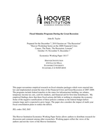
such as aid to the states or temporary tax rebates—used during these years, with less emphasis onmodels. I also examine some journalistic interpretations of research and the use of modelsdesigned specifically to estimate the impact of long-term credible fiscal consolidation plans.1. Macro Model Estimates of the Impacts of Fiscal Stimulus in 2007-09 RecessionStructural macroeconomic models are natural starting point for the evaluation of fiscalpolicy. Policy simulations with such models can help estimate the impact of actual fiscalstimulus packages and thereby determine whether such policies are appropriate.When estimating the impacts of fiscal policy, however, different macro models can givedifferent answers. Figure 1 illustrates of how large the differences can be, at least as seen fromthe vantage point of 2008. It shows two estimates from two different macro models of theimpact of a one-time permanent increase in government spending on real GDP in the UnitedStates. One type of model—often called new Keynesian—endeavors to incorporate thebehavior of forward-looking agents who try to anticipate changes in policy and adaptaccordingly. The other type of model, which might be called old Keynesian for contrast, does notincorporate forward looking behavior and assumes that expectations adapt slowly over time.Both types of models incorporate rigidities such as sticky wages and prices.3
Figure 1. Estimated Impact on Real GDP of a Permanent Increase inGovernment Purchases of 1 percent of GDPThe path labeled “Romer and Bernstein (2009)” in Figure 1 is based on an averagecomputed by Romer and Bernstein (2009) in January 2009 of models of the old Keynesianvariety that were used by the staff of the Federal Reserve Board and a private forecasting firm atthat time. It shows the estimated impact of an unanticipated permanent increase in governmentpurchases of 1 percent of GDP; according to this type of model, the policy would lead to anincrease in real GDP of 1.6 percent. Figure 1 also shows the estimated effect of the exact samepolicy change—a permanent increase in government purchases—using a model of the newKeynesian type developed by Taylor (1993) which also existed at that time. It is clear fromFigure 1 that the two approaches imply vastly different results. In one case higher government4
spending keeps on adding to GDP, while in the other case the effect on GDP diminishes quicklyas non-government components are crowded out by government spending.In assessing the effect of government actions on the economy, it is of course important tomodel how households and firms adjust their spending decisions as their expectations of thefuture changes. Because new Keynesian models endeavor to capture how people’s expectationsand economic behavior change over time in response to policy interventions, they are moresuitable for estimating the effects of policy. For this reason, they are often taught in economicsgraduate schools and are a foundation upon which improvements are considered in research. Wefocus on new Keynesian models in this review. This focus reduces, but does not eliminate, as Iwill show, the differences between models. A very important topic for future research is theexamination of the impact of fiscal stimulus packages using improved new Keynesian modelsincluding those that deal with heterogeneous agents as in Auclert (2017) or Kaplan, Moll, andViolante (2018).Consider the impact of the 2009 stimulus package using the new Keynesian SmetsWouters model of the U.S. economy, one of the best known of the empirically-estimated newKeynesian models. It is very similar to another well-known empirically-estimated newKeynesian model developed by Christiano, Eichenbaum and Evans (2005) (CEE) and has beencited by Woodford (2009) as a leading model in a review of current thinking in macroeconomics.What does this model imply about the impact of the 2009 fiscal stimulus package?Cogan, Cwik, Taylor and Wieland (2010) (CCTW) answered this question by simulating thefiscal stimulus package enacted and signed into law on February 17, 2009; the results aresummarized in Cogan, Taylor, and Wieland (2009). The stimulus package was a mixture ofhigher government purchases, increased transfer payments, and tax refunds. In fact, about half of5
that stimulus package consisted of transfer payments (for unemployment assistance, nutritionalaid, health and welfare payments, and temporary tax cuts). Another component was federalgovernment transfers to state and local governments to be used for the purchase of goods andservices and build infrastructure.Figure 2 presents the results of the simulation showing the impact of the change ingovernment purchases. The bar graph shows how much government purchases increased as ashare of GDP, and the line graph shows the impact of the increase in purchases on real GDP inthe Smets-Wouters model.Figure 2. Impact of the 2009 stimulus package based on the Smets-Wouters modelAccording to the Smets-Wouters model, the estimated impacts on GDP are very small,with the multiplier well below one. Note that during the first year the estimated stimulus is6
minor and then even turns down in the third quarter. Why is the effect so small in the first year?The answer comes in part from the timing of the government expenditures and the forwardlooking perspective of households. The small amount of government spending in the first year isfollowed by a larger increase in the second year. Households and firms anticipate the secondyear increase during the first year. They also anticipate that ultimately the expenditures will befinanced by higher taxes. The negative impact of the delayed government spending and thenegative wealth effect on private consumption of higher anticipated future taxes combine toreduce the positive impact of the stimulus. As a result, the first-year GDP impact is initiallysmall and turns down.In the Smets-Wouters model there is also a strong crowding out of investment. Hence,both consumption and investment decline as a share of GDP in the first year according to themodel. This negative effect is offset, as shown in Figure 2, by the increase in governmentspending in the first year, but it causes the multiplier to be below one right from the start.Of course, not all new Keynesian models are the same as the Smets-Wouters model; thereare different views of the theoretical framework and econometric methodology. But howdifferent are the estimated results of the fiscal stimulus packages? An answer is proved in thepaper, “Effects of Fiscal Stimulus in Structural Models,” written by economic researchers atcentral banks and international institutions around the world (Guenter Coenen, Chris Erceg,Charles Freedman, Davide Furceri, Michael Kumhof, René Lalonde, Douglas Laxton, JesperLindé, Annabelle Mourougane, Dirk Muir, Susanna Mursula, Carlos de Resende, John Roberts,Werner Roeger, Stephen Snudden, Mathias Trabandt, and Jan in’t Veld). The authors comparedthe Smets-Wouters model estimates of the 2009 stimulus package with the CEE model, used inChristiano, Eichenbaum, and Rebelo (2011), and four other new Keynesian structural7
macroeconomic models of the kind used in practice by policymakers and their staffs. The otherfour models are the Bank of Canada’s GEM model (BOC), the Fed’s FRBUS model (FRB), theFed’s SIGMA model (SIGMA), and the International Monetary Fund’s GIMF model (IMF).Coenen et al. (2012) simulated all 6 models using same time profile of governmentpurchases used by CCTW to describe the American Recovery and Reinvestment Act of 2009(ARRA). The estimates, of course, depend on the monetary policy rule used in the model. Theresults for GDP are shown in Figure 3 (which corresponds to Figure 7 of Coenen et al. (2012))and refers to the estimates with the assumption of two full years of monetary accommodationduring which the central bank keeps the interest rate near zero. Observe that the four policymodels give estimates very similar to those of CCTW, though the CEE model appears to be anoutlier.Figure 3. Estimates of Fiscal Stimulus based on Simulations of Different Macro Models8
Given the range of variation in Figure 1, one wonders where the idea came from thatthere was a consensus that the stimulus was very effective as mentioned by Phelps (2018). Oneanswer is that journalistic and popular reporting sometimes characterized the situationdifferently. A good example is a November 2009 article in the New York Times with the headline“New Consensus Sees Stimulus Package as a Worthy Step.” (Calmes and Cooper (2009)). Thearticle noted that “the accumulation of hard data and real-life experience has allowed moredispassionate analysts to reach a consensus that the stimulus package, messy as it is, is working.The legislation, a variety of economists say, is helping an economy in free fall a year ago to growagain and shed fewer jobs than it otherwise would.”As evidence, the article included three graphs, which are reproduced on the left of Figure4. Each of the three graphs on the left corresponds to a model maintained by the modelling groupshown above the graph. All three graphs show that without the stimulus economic growth wouldbe considerably weaker. The difference between the black line and the gray line is theirestimated impact of the stimulus.Now what about the so-called “consensus?” In fact, as is clear from the previousdiscussion, other economic models estimated that the stimulus was not very effective. Toillustrate this, I have added two other graphs on the right-hand side of Figure 4 which did notappear in the New York Times article. The first one is based on the Smets-Wouters modelsimulations discussed above. Focus on the difference between the black and the gray lines, whichis what is predicted by that model, which shows that the impact is very small. The secondadditional graph on the right is based on the research of Barro (2009) about which he explained,“when I attempted to estimate directly the multiplier associated with peacetime governmentpurchases, I got a number insignificantly different from zero.” So according to that research, the9
difference between the black and the gray line should be about zero, which is what that graphshows. In sum, there is no consensus after all.Figure 4. Evaluation of stimulus packages: 3 models from NYT article and 2 alternatives.Some algebra will help show what is going on. Consider two models relating the size ofthe stimulus package S to output Y. Model A is Y αS Z and Model B is Y Z, where Z is anunobservable shock and α is a coefficient which we set to 1.5. Now, suppose that a stimulus isenacted with S 2, but Y decreases by -1. Then the shock implied by Model A is Z - 4 whilethe shock implied by model B is Z -1.Now consider policy evaluation of the stimulus based on a counterfactual where there isno stimulus so S 0. Economists using Model A would say: “Just as we predicted, the stimuluspackage worked. Without it, Y would have fallen to -4 rather than -1. The decline in outputwould have been 4 times as deep, a Great Depression 2.0.” Economists using Model B wouldsimply say “Just as we predicted the stimulus package did not work.”10
2. The Direct Macroeconomic Estimates of the Impact of Fiscal Stimulus ProgramsOne way to address the problem of differing models is to look at data on the direct effectof the stimulus packages without imposing a rigid model structure. First, I look at the effect ofthe temporary transfers and tax rebates in the 2001, 2008, and 2009 stimulus packages onconsumption. Then I consider the impact of government purchases. The approach used herefocuses on stimulus-specific timing and compositional effects which help in identifying theimpacts of the policy changes.Temporary Tax cuts and RebatesThe macroeconomic theory that rationalizes such temporary payments holds that theyincrease the demand for consumption, stimulate aggregate demand, and thereby help get theeconomy on a path to recovery. Counterarguments arise from doubts about the reliability andstability of the connection between income and consumption, especially when the increase inincome due to the stimulus is temporary.What do the data show? First consider the 2008 rebate for which we have monthly dataas described in Taylor (2009). Figure 5 illustrates the impact on consumption. The upper lineshows disposable personal income for the months from January 2007 through October 2008.The data are seasonally adjusted and are stated at annual rates. Disposable personal income isthe total amount of income after taxes and government transfers; it therefore includes the rebatepayments. Subtracting the rebate payments from the top line results in the dashed line in Figure5, which shows what disposable personal income would have been without the rebates. Noticethe sharp increase in disposable personal income in May 2008 when rebates were mailed ordeposited in people’s bank accounts. Disposable personal income then started to come down in11
June and July as total payments declined and by August had returned to the trend that wasprevailing in April.The lower line in Figure 5 is personal consumption expenditures over the same period.Observe that consumption shows no noticeable increase at the time of the rebate. As the pictureillustrates the temporary rebate did little or nothing to stimulate consumption demand, andthereby aggregate demand, or the economy. In fact, the data show that consumption begandeclining in July 2008 and continued to decline through October.Figure 5. Income, Consumption, and the 2008 Rebate PaymentsNow compare the tax and transfer components of the 2001, 2008 and 2009 stimuluspackages using quarterly data. Figure 6 shows the impact on quarterly disposable personalincome of the temporary changes in taxes and transfers due to the three stimulus packages of the12
2000s as calculated in Taylor (2011). The impacts of the packages on income were calculated byBEA. For the 2001 and 2008 packages the data were collected from various monthly BEA pressreleases of “Personal Income and Output.” For the 2009 package the data were collected in asatellite quarterly account on ARRA prepared by BEA, “Effect of the ARRA on Selected FederalGovernment Sector Transactions” under the categories “personal current taxes” or “currenttransfer payments to persons.” These changes include one-time 250 payments, refundablecredits, and a “making work pay” tax credit.Figure 6Though these packages differed in size, duration, and the mechanism for distribution ofthe stimulus payments, they were quite similar from the point of view of macroeconomics13
because they were all widely viewed as temporary and were justified on the grounds ofstimulating or jump-starting consumption. In fact, a big idea underlying the 2008 and 2009stimulus packages was that they should be temporary, as well as targeted and timely. Thistemporary feature distinguishes these actions from more permanent changes such as the personalincome tax rate cuts of the 1980s.Now consider the impact of these temporary changes in disposable personal income onconsumption. It would be too narrow an interpretation of the macro theory to say thatconsumption would adjust perfectly in synch with the ups and downs in income due to thepayments. But if the stimulus payments worked to stimulate the economy as envisioned in thismodel, one would have to see some associated movements in consumption. To look for suchdirect effects, I subtracted the payment amounts in Figure 6 from actual disposable personalincome to get an adjusted income series as shown in Figure 7 for the 2008 and 2009 stimuluspackages. The actual and adjusted series can then be compared with personal consumptionexpenditures also shown in Figure 7.14
Figure 7Figure 7 does not reveal any noticeable effects of the temporary payments onconsumption. The sharp increases in personal disposable income in the second quarter of 2008and the second quarter of 2009 do not show up in movements in consumption. Recall that thelack of a relationship is even more striking with monthly data as shown in Figure 5.More precise information about the direct impact of the stimulus payments onconsumption can be obtained from regression estimates. Table 1 reports the results from threeregressions in which personal consumption expenditures (PCE) is the left-hand side variable. Inregression equation 1, displayed in column 1, the income variable is simply disposable personalincome (which includes the stimulus). In the second regression equation, the income variable isdisposable personal income without the stimulus. In the third equation, the stimulus payments for15
2001, 2008 and 2009 are added as a separate variable. In all three regressions, oil prices andhousehold net worth are included as control variables. Higher oil prices would be expected todepress consumption while higher net worth should have a positive effect, both with some lag,and this is what the regressions show with the lag equal to two quarters.By choosing to put consumption on the left-hand side, we are looking for effects of thestimulus payments on consumption, which is where most macro theories say we should findthem. By splitting disposable personal income into two parts—a temporary part due to thestimulus and the remaining more permanent part—we are allowing for a distinction predicted bythe permanent income theory, though we are not prejudging the size of the temporary versuspermanent effect. The regressions are estimated over the sample period 2000Q1- 2011Q1 whichincludes the effects of all three stimulus packages.First note that the standard error in regression equation 2 is less than the standard error inregression equation 1. In other words, including the stimulus payments in disposable personalincome worsens the fit of the equation, suggesting that the impact of the temporary changes onconsumption is less than the more permanent changes. This idea is borne out by comparingequation 2 with equation 3 where the stimulus payment is separated from other sources ofincome. Regression equation 3 indicates that the temporary stimulus payments had a very smalleffect on consumption and that this effect is not statistically significantly different from zero. Incontrast, the adjusted disposable personal income variable—a more permanent measure ofincome—has a much larger and statistically significant effect in regression equation 3.This is the kind of regression result that one would expect from Milton Friedman’spermanent income hypothesis, Franco Modigliani’s life cycle hypothesis or from consumptionsmoothing in an inter-temporal utility maximization model. Experimenting with different16
regression specifications gives similar results, so effectively the data are speaking for themselveswithout the constraint of a model or functional form. The results imply that the Keynesianmultiplier for transfer payments or temporary tax rebates was not significantly different fromzero for the kind of stimulus programs enacted in the 2000s.17
Table 1—Quarterly PCE Regressions With and Without Stimulus 1(-.25)Disposable PersonalIncome.817(40.9)--------Disposable PersonalIncome--Without Stimulus----.857(73.0).851(60.4)Stimulus Payments----------0.128(0.81)Oil Price ( /bbl lagged 2 quarters)-2.41(-4.71)-2.55(-4.14)-2.55(-4.61)Net Worth (lagged 2 quarters).021(8.53).017(7.32).018(7.97)Standard error of regression76.965.866.3Note: The dependent variable is personal consumption expenditures (PCE). The t-statistics inparentheses are based on Newey-West standard errors. The oil price variable is West TexasIntermediate and net worth variable is Household Net Worth from the Flow of Funds, Table B100, line 42. Sample period is 2000Q1 - 2011Q1.Government Purchases and Infrastructure Spending in the 2009 Stimulus ActNow consider the impact of changes in government purchases. The 2001 and 2008stimulus programs did not have a government purchases component, so we focus on the 2009stimulus package. Figure 8 summarizes the impact of the stimulus legislation on federalgovernment sector transactions from 2009.1 to 2011.1. Three components are shown:1.The temporary transfers and tax rebates or credits which increase the disposablepersonal income of individuals and families.18
2.Federal government purchases of goods and services (government consumptionand government investment) and3.Federal grants to states and local governments.The second category, federal government purchases of goods and services, is part ofGDP and thereby contributes directly to changes in GDP. The amount by which an increase ingovernment purchases in a stimulus package raises GDP is of course the government purchasesmultiplier. From a fiscal stimulus perspective, the purpose of the third category—sending grantsto state and local governments—is to get these governments to increase purchases.As shown in Figure 8, only a small part of the 2009 stimulus went to purchases of goodsand services by the federal government. At the maximum effect, which occurred in the thirdquarter of 2010, federal government purchases due to ARRA reached only 0.21 percent of GDPand federal infrastructure only 0.05 percent of GDP.These amounts are too small for the stimulus package to have had a significant effect onthe overall economy. In this case the debate over the size of the government purchasesmultiplier is largely moot because the government purchases multiplier had virtually nothing tomultiply at the federal level.19
Figure 8State and local governments received substantial grants under ARRA as shown in the barchart. The purpose of sending these grants to the states was to encourage them to undertakeinfrastructure projects and purchase other goods and services. But this is not what happened.Consider Figure 9 which shows the stimulus grants along with the change in state andlocal government purchases, borrowing, and expenditures other than government purchasesrelative to the fourth quarter of 2008. Stimulus grants increased steadily from the first quarter of2009 through the third quarter of 2010 before tapering off. But as shown by Cogan and Taylor(2011, 2012), state and local government purchases hardly changed at all during this period. Thebiggest change during the period of the stimulus grants was a large decrease in net borrowing bystate and local governments, or, equivalently, an increase in net lending. Expenditures other than20
the purchases of goods and services rose by a smaller amount than net lending. Net borrowing bythe state and local government sector is defined as the difference between the net increase infinancial liabilities and the net acquisition of financial assets or equivalently by totalexpenditures less total revenues.Figure 9To get a better estimate of the direct impact of the ARRA grants on governmentpurchases Cogan and Taylor (2012) used regression methods to control for other state and localgovernment revenues (excluding ARRA grants) and also to take account of the state and localgovernment budget constraint. By imposing the budget constraint on the regression coefficients,we let the data determine what component of the budget the ARRA grants affected and by how21
much. We found that the direct effect of ARRA grants was to lower net borrowing by the sameamount as these ARRA grants, so they had no effect on the sum of purchases and otherexpenditures.Some argue that the economy would have been worse off without these stimuluspackages, but the results do not support that view. If there had been no ARRA grants to statesand localities, their total expenditures would have been about the same. The counterfactualsimulations show that the ARRA-induced decline in state and local government purchases waslarger than the increase in federal government purchases due to ARRA. In terms of the simpleexample of Model A versus Model B presented above, these results are evidence against theviews represented by Model A, and thus against using such models to show that things wouldhave been worse.Others, including Stiglitz (2018), argue that the stimulus was too small, but the results donot lend support to that view. Using the estimated equations, a counterfactual simulation of alarger stimulus package—with the proportions going to state and local grants, federal purchases,and transfers to individual the same as in ARRA—would show little change in governmentpurchases or consumption, as the temporary funds would be largely saved. Of course, the storywould be different for a stimulus program designed more effectively to increase purchases, but itis not clear that such a p
federal debt to new records. Accordingly, the paper also considers the impact of multi-year fiscal consolidation plans to reduce the deficit. The focus here is on macroeconomic analysis. I first review research that uses macroeconomic models to estimate the impact of demand-side stimulus packages. I then