WIXLIB

Figure 4: Per movie (a) and user (b) standard deviation(std) in Netflix and Rotten Tomatoesa mean rating 0.4 (2 ), but the range 0.8 to 1 alsoaccounts for 10% of the movies.In a similar way, Figure 3b shows that the user ratingshave a normal distribution centered around 0.7 (4 ) whileexpert ratings are centered around 0.6 (3.5 ). Note that inthis case, only 10% of the users have a mean score 0.55and another 10% 0.7. In terms of how the average ratingis distributed, we see that experts show greater variabilityper movie than per user: while experts tend to behave similarly in terms of their average rating, their overall opinionon the movies is more varied. This could be due to underlying incentives to rate movies, since experts are likely towatch and rate movies regardless of whether they like themor not, while users tend to be biased towards positively rating movies [5]. We also detect a much larger proportion ofmovies in the highest rating range for experts. Experts seemto consistently agree on what the “excellent” movies are.Rating Standard Deviation (std). Figures 4a and 4bplot the distribution of the std per movie (a) and user (a)in Netflix and Rotten Tomatoes, respectively. In the case ofusers, the std per movie (Figure 4a) is centered around 0.25(1 ) with very little variation, while the expert data set hassignificantly lower std (0.15) and larger variation. Note thatin the expert data, 20% of the items show no std as thereis only one rating. The std per user (Figure 4b) is centeredaround 0.25 for the Netflix data with larger variability thanin the per movie case. When looking at the expert data, theaverage std per user is 0.2 with small variability.The above analysis highlights the large differences between our user and expert sets. The expert data set is muchless sparse than the users’. Experts rate movies all over therating scale instead of being biased towards rating only popular movies. However, they seem to consistently agree onthe good movies. Experts also have a lower overall standarddeviation per movie: they tend to agree more than regularusers. Also, the per-expert standard deviation is lower thanthat seen between users, meaning that they tend to deviateless from their personal average rating.3.EXPERT NEAREST-NEIGHBORSThe generic CF method applies the kNN algorithm to predict user ratings. The algorithm computes a prediction fora user-item pair, based on a number k of nearest neighbors,which can either be user- or item-based [6]. Although it ispossible to use either approach, we choose user-based CF forits transparent applicability to experts. Both approachescan be decomposed into a sequence of stages. In the firststage, a matrix of user-item ratings is populated. Then, thesimilarity between all pairs of users is computed, based ona pre-determined measure of similarity. In a similar way towhat Herlocker et. al propose [7], we use a variation of thecosine similarity which includes an adjusting factor to takeinto account the number of items co-rated by both users.Given users a and b, item i, user-item ratings rai and rbi ,the number of items Na and Nb rated by each user, and thenumber of co-rated items Na b the similarity is computedas:Pi(rai rbi )2Na bsim(a, b) qPqP·(1)Na Nbi 2i 2rairbiWe propose an approach to CF that only uses expert opinions to predict user ratings. Therefore, our approach doesnot require the user-user similarity to be computed; instead,we build a similarity matrix between each user and the expert set. We take a slightly different approach than regular k -NN CF. Our expert-CF method is closely related toMa et al.’s method for neighborhood selection [8]. In order to predict a user’s rating for a particular item, we lookfor the experts whose similarity to the given user is greaterthan δ. Formally: given a space V of users and expertsand a similarity measure sim : V V R, we define aset of experts E {e1 , ., ek } V and a set of usersU {u1 , ., uN } V . Given a particular user u Uand a value δ, we find the set of experts E ′ E such that: e E ′ sim(u, e) δ.One of the drawbacks of using a fixed-threshold δ is therisk of finding very few neighbors; furthermore, the ones thatare found may not have rated the current item. In order todeal with this problem, we define a confidence threshold τas the minimum number of expert neighbors who must haverated the item in order to trust their prediction. Given theset of experts E ′ found in the previous step and an item i,we find the subset E ′′ E ′ such that e E ′′ rei 6 ,where rei is the rating of item i by expert e E ′ , and isthe value of the unrated item.Once this subset of experts E ′′ e1 .en has been identified, if n τ , no prediction can be made and the user meanis returned. On the other hand, if n τ , a predicted ratingcan be computed. This is done by means of a similarityweighted average of the ratings input from each expert e inE ′′ [9]:Pe E ′′ (rei σe )sim(e, a)P(2)rai σu sim(e, a)where rai is the predicted rating of item i for user a, rei isthe known rating for expert e to item i, and σu and σe arethe respective mean ratings.In the next section, we report on the interplay of the twoparameters δ and τ . The optimal setting of these parameters depends on the data set and the application in mind,as it is the case with other state-of-the-art CF algorithms.Also, and in order to make our results comparable, note thatwe use the same threshold-based nearest-neighbor approachwhen comparing with the standard CF method.4. RESULTSBased on the previously described data, we measure howwell the 169 experts predict the ratings of the 10, 000 Netflixusers. In order to validate our approach, we set up two different experiments: in the first experiment, we measure themean error and coverage of the predicted recommendations.In the second experiment, we measure the precision of the

MethodCritics’ ChoiceExpert-CFN Table 1: Summary of the MAE and Coverage in our Expertbased CF approach compared to Critics’ Choice and Neighbor CFrecommendation lists generated for the users.4.1 Error in Predicted RecommendationsIn order to evaluate the predictive potential of expert ratings, we divided our user data set (by random sampling)into 80% training - 20% testing sets and report the average results of a 5-fold cross-validation. We use the averagefor all experts over each given item as a worst-case baselinemeasure. This is equivalent to a non-personalized “critics’choice” recommendation, which produces a Mean AverageError (MAE) of 0.885 and full coverage. Setting our parameters to τ 10 and δ 0.01, we obtain a MAE of0.781 and a coverage of 97.7%. Therefore, expert-CF yieldsa significant accuracy improvement with respect to using theexperts’ average. As far as coverage is concerned, the settingof the parameters represents a small loss. We shall turn nextto the details of how the two parameters in our approach (δor minimum similarity and τ or confidence threshold) interplay.Figure 5a shows that the MAE in the expert-CF approachis inversely proportional to the similarity threshold (δ) until the 0.06 mark, when it starts to increase as we moveto higher δ values. The accuracy below the 0.0 thresholddegrades rapidly4 , as we are taking into account too manyexperts; above 0.06, though, we have too few experts inthe neighborhood to make a good prediction. If we lookat Figure 5b we see how it decreases as we increase δ. Forthe optimal MAE point of 0.06, coverage is still above 70%.The ultimate trade-off between MAE and coverage will beapplication-specific. Turning to Figure 5c, we see how theMAE evolves as a function of the confidence threshold (τ ).The two depicted curves correspond to δ 0.0 and δ 0.01.We choose these two values of our similarity threshold asthey produce a reasonable tradeoff between accuracy andcoverage.Standard neighbor-CF (ignoring the expert data set) offers a second baseline measure of performance. A side-toside comparison gives us a first intuition.Using the Netflix users as neighbors, we measure a MAEof 0.704 and 92.9% coverage when the δ 0.01 and τ 10(see summary in Table 1) 5 . Figure 6 includes a detailedcomparison of the accuracy and coverage of the expert-CF(experts line) and NN-CF (neighbors) methods as a functionof the similarity threshold. While NN-CF has a MAE 10%lower than expert-CF, the difference in their coverage is alsoaround 10%, favoring the experts in this case.4Note that this threshold values are dependent on the chosensimilarity measure. In our case, we are using a symmetriccosine similarity that can yield values between [ 1, 1].5It should be noted, for consistency sake, that using thisparameters yields very similar results to standard k NN CFwith k 50, which is a common setting [10]. In this casewe measure a MAE of 0.705.Finally, we are interested in measuring whether the difference in prediction accuracy is equally distributed among alltarget users. Figure 6b includes the cumulative distributionof per-user error for both methods. Note how both curvesseparate at around MAE 0.5 and they run almost parallelwith a separation of around 0.1 until they start joining againat around the point of MAE 1. This means that neighborNN works better for the minority of users with a low MAEaverage of less than 0.5, which represent around 10% of ourpopulation. Both methods perform equally the same for therest of the users – with the expert-CF approach performingeven slightly better for users with a MAE higher than one.This is a positive feature of our approach that only performsworse on users that are highly predictable, in which a slightincrease in error should be acceptable.4.2 Top-N Recommendation PrecisionAlthough measuring the mean error on all predictions fora test data set is currently an accepted measure of successfor recommender systems, we are interested in evaluatingour results in a more realistic setting. A “real-world” recommender system only recommends the set of items that theuser may like. This is similar to the idea of top-N recommendation lists [11].The evaluation of recommendation algorithms throughtop-N measures has been addressed before [12, 13]. All ofthese approaches rely on the use of the well-known precisionand recall measures. Ziegler et al. show [14] that evaluatingrecommender algorithms through top-N lists measures doesnot map directly to the user’s utility function. However, itdoes address some of the limitations of the more commonlyaccepted accuracy measures, such as MAE.We propose a variation as an extension to the previouslydescribed approaches. In our case, we do not construct thelist of recommendable items by fixing N , but rather classifyitems as being recommendable or not recommendable givena threshold: if there is no item in the test set that is worthrecommending to a given target user, we simply return anempty list. We believe that using a recommendable threshold is a more appropriate measure for top-N recommendations than, for instance, the ones proposed by Deshpandeand Karipis [11], where the user rating was not taken intoaccount in the evaluation process. The most similar approach to ours is that proposed by Basu et al. [15], wherethey use the top quartile of a user’s ratings in order to decide whether a movie is recommendable. We do not use themodified precision measure proposed in [13] for two reasons:First, because we believe it is unfair with algorithms thatpromote serendipity. And second, and most important, because we will later do a final validation with a user studyin which we will use the same procedure for generating thelists. In that setting, we will aim at recommending previously unrated items. Therefore, penalizing unrated items asproposed in the modified precision would make both resultsnot comparable.Therefore, we define an item to be recommendable if itspredicted value is greater than σ. With this definition inmind, we evaluate our system as a 2-class classification problem:1. For a given user, compute all predictions and presentthose greater or equal than σ to the user2. For all predicted items that are present in the user’s

(a) MAE vs. similarity threshold(b) Coverage vs. similarity threshold(c) MAE vs. ConfidenceFigure 5: (a) Mean absolute error (MAE) and (b) coverage of expert-predicted ratings as a function of the minimum similarity(δ) and confidence (τ ) thresholds; (c) MAE versus confidence threshold.User Error Distribution0.6neighbors experts0.20.4Cumulative Distribution0.80experts0.75Mean Absolute Error0.80.851.0Effect of Similarity Threshold0.700.0neighbors 0.020.000.020.040.060.080.100.120.00.5Similarity Threshold1.01.52.02.5User Mean Absolute Error(a)(b)Figure 6: Comparison between Expert CF and Nearest-Neighbor CF: (a) MAE and (b) per user error.Precision Comparison0.951.00test set, look at whether it is a true positive (actualuser rating greater or equal to σ) or a false positive(actual user rating less than σ).0.90neighbors0.85experts0.80We measure a precision of 0.76 using the same parametervalues reported in Section 4.1 and setting σ 4. This meansthat 76% of the items recommended by the experts found inthe user test set are qualified as recommendable by the users.Note, however, that a recommendable threshold of 4 is quiterestrictive. If we lower σ to 3, we measure a precision of 89%.Figure 4.2 depicts the variation of the precision of NN-CF(neighbors line) and expert-CF (experts line) with respect toσ. For σ 4, the baseline method clearly outperforms ourexpert-based approach with a precision of 0.85. However, forσ 3 the precision in both methods is similar. Therefore,for users willing to accept recommendations for any aboveaverage item, the expert-based method appears to behaveas well as a standard NN-CF.Precision3. Compute the precision of our classifications using theclassical definition of this measure1.01.52.02.53.03.54.0Recommendable ThresholdFigure 7: Precision of Expert CF (experts line) as comparedto the baseline NN CF (neighbors line) as a function of therecommendable threshold σ.

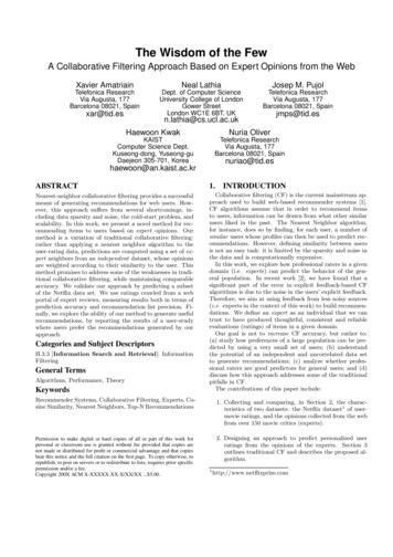
5.USER STUDYAlthough error and recommendation list precision are prominent metrics used for CF evaluation, their relation to theactual quality of the recommendation is unclear. Therefore,we designed a user study to further validate our findings. Wedesigned a web interface that asked users to rate 100 preselected movies. The selection was done by using a stratifiedrandom sample on the movie popularity curve: we dividedthe 500, 000 Netflix movies into 10 equal-density bins andrandom sampled 10 movies from each bin. We provideda “have not seen” button so users could voluntarily decidewhich movies to rate.57 participants were recruited via email advertisement ina large telecommunications company. The participants’ ageranged from 22 to 47 years, with an average age of 31.2 years.Almost 90% of our participants were in the 22 to 37 agegroup and most of them were male (79.12%). Note, however,that this demographic group corresponds to the most activegroup in online applications such as recommender systems[16].Using the collected ratings and the 8, 000 movies that weconsidered in the above experiments, we generated 4 top-10recommendation lists: (i) Random List: A random sequence of movie titles; (ii) Critics choice: The movieswith the highest mean rating given by the experts. If twomovies had the same mean, we ranked them based on howmany experts had rated the movie; (iii) Neighbor-CF:Each survey respondents’ profile was compared to the ratings of the users in the Netflix data subset: the top-10 listwas derived by ordering the unrated movies with predictions higher than the recommendable threshold; and (iv)Expert-CF: Similar to (iii), but using the expert datasetinstead of the Netflix ratings.Both neighbor-CF and expert-CF used the same settings:a similarity threshold of 0.01 and a confidence measure of 10.Note that, as we saw in Figure 6, the setting of a given similarity threshold is not unfair to any of the two approaches.Therefore, we choose a value that gives us enough coverageso as to produce enough recommendations. For the settings we chose, the RMSE values are the ones we includedin Table 1. Increasing the similarity threshold would reducecoverage, while the ratio between both RMSE’s would remain the same. Increasing the confidence threshold wouldalso reduce coverage. Note that the neighbor-CF algorithmwould be especially sensitive to changes in the confidencethreshold. The coverage of neighbor-CF is 92.9% with thecurrent setting of the threshold, compared to 97.7% in thecase of expert-CF. Also note that, as already explained inthe previous section, these settings for the neighbor-CF yieldan error comparable to standard k NN with k 50.We then asked our participants to evaluate: (i) The overall quality of the recommendation lists; (ii) whether theyincluded items that the user liked; (iii) whether they included items that the user did not like; and (iii) whetherthey included surprising items.The average number of ratings was of 14.5 per participant. We had to generate the recommendation lists basedon such limited user feedback. Therefore, our test conditions are similar to a real setting where the user has recentlystarted using the recommendation service. Our results arethus assessing how well the methods perform in cold-startconditions.Figure 8 includes the responses to the overall list quality.““(a)(b)Figure 9: User study responses to whether the list containsmovies users would like or would not like.Participants were asked to respond in a 1 to 5 Likert scale asthe one included in Figure 8a. Note that we also report theaveraged results in Figure 8b. We can see that the expert-CFapproach is the only method that obtains an average ratinghigher than 3. Interestingly, the standard neighbor-CF approach performs almost as badly as a randomly generatedlist. The only approaches that are qualified as very goodare expert based: critics’ choice and expert-CF. In addition,50% of the users considered the expert-CF recommendationsto be good or very good. Finally, it is important to stressthat although an average rate of 3.4 might seem low, this isin a cold-start situation with very limited information fromeach user.In Figure 9 we report on the replies to the question ofwhether participants felt the generated lists contained itemsthey knew they would like/dislike. In these cases, we useda 1 to 4 Likert scale, removing the neutral response. Wereport average results for clarity. In Figure 9a, we againsee that the expert-CF approach outperforms the rest ofthe methods. More than 80% of the users agreed (or fullyagreed) that this method generates lists that include moviesthey like. It is interesting to note that this figure is similarto the assessed overall list quality in Figure 8b.Figure 9b summarizes the ratings to the question ”the listcontains movies I think I would not like”. This questionis very important: recommending wrong items mines theuser’s assessment of the system and compromises its usability [17]. Therefore, an important aspect on the evaluation ofa recommender system is how often the user is disappointedby the results. The expert-CF approach generates the leastnegative response when compared to the other methods.Finally, we performed an analysis of variance (anova) totest whether the differences between the four recommendation lists are statistically significant or not. The null hypothesis is that the average user evaluation for the four differentlists is the same. The confidence level is set to 99%, suchthat p-values smaller than 0.01 imply a rejection of the nullhypothesis. The p-value for the fours lists is 5.1e 05 andconsequently the null hypothesis is rejected. If we leave outthe expert-CF algorithm from the analysis, we measure a pvalue of 0.42. In this case, we conclude that the differenceson the user satisfaction from the three baseline methods isnot statistically significant. The cross-comparison betweenthe expert-CF and the other three algorithms gives p-valuesof 2.14e 05, 2.4e 03 and 8e 03 for Random, neighborCF and Critics’ Choice respectively. From these results, we

(a) Comparison of the responses to overall quality of the recommendation lists generated by 4 methods.(b) Overall quality of the expert-CF method as compared to others, average responseFigure 8: Overall quality of different recommendation strategies as assessed by our user study participants.conclude that the differences on the participants’ satisfactionproduced by the expert-CF algorithm cannot be attributedto the sampling of the user study.6.DISCUSSIONIn this paper, we have introduced a recommender systemthat uses a small set of expert ratings to generate predictions for a large population of users. Our experiments arebased on using online reviews from movie critics. However,we could also think of a small set of “professional” ratersmaintaining a rating database. This is reminiscent but lessdemandi

watch and rate movies regardless of whether they like them or not, while users tend to be biased towards positively rat-ing movies [5]. We also detect a much larger proportion of movies in the highest rating range for experts. Experts seem to consistently agree on what the"excellent"movies are. Rating Standard Deviation (std). Figures 4a and 4b