Transcription
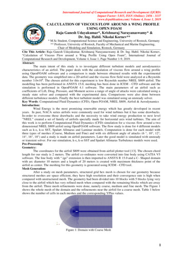
International Journal of Computational Research and Development (IJCRD)Impact Factor: 5.015, ISSN (Online): 2456 - 3137(www.dvpublication.com) Volume 4, Issue 1, 2019CALCULATION OF VISCOUS FLOW AROUND A WING PROFILEUSING OPEN FOAMRaja Ganesh Udayakumar*, Krishnaraj Narayanaswamy* &Dr. Ing. Habil. Nikolai Kornev*** M.Sc Student, Computational Science and Engineering, University of Rostock, Germany** Professor, University of Rostock, Faculty of Mechanical and Marine Engineering,Chair of Modeling and Simulation, Rostock, GermanyCite This Article: Raja Ganesh Udayakumar, Krishnaraj Narayanaswamy & Dr. Ing. Habil. Nikolai Kornev,“Calculation of Viscous Flow around a Wing Profile Using Open Foam”, International Journal ofComputational Research and Development, Volume 4, Issue 1, Page Number 1-9, 2019.Abstract:The main intent of this study is to investigate different turbulent models and aerodynamicscharacteristics of an airfoil. The paper deals with the calculation of viscous flow around a wing profileusing OpenFOAM software and a comparison is made between obtained results with the experimentaldata. The geometry was simplified into a 2D airfoil and the viscous flow field were analyzed at a Reynoldsnumber 3.0 106. The chosen airfoil for this experiment is low Reynolds number NREL S809 airfoil. Themodelling has been performed in ANSYS 15.0, meshing has been done in ICEM - CFD software and thesimulation is performed in OpenFOAM 4.1 software. The main parameters of an airfoil such ascoefficients of Lift, Drag, Pressure, and Moment across a range of angle of attacks were calculated using asteady state solver and compared with the experimental data. Comparisons were also done betweendifferent turbulence models. Finally the best turbulent model was simulated using an unsteady solver.Key Words: Computational Fluid Dynamics (CFD), Open FOAM, NREL S809, Airfoil & AerodynamicsIntroduction:Wind Energy is the most promising renewable energy which has greatly developed in recentyears. In past, NACA series airfoils were commonly used for wind turbines but it has some drawbacks.In-order to overcome those drawbacks and the necessity to take wind energy production to next level”NREL” created a set of family of airfoils specially made for horizontal axis wind turbines. The aim ofthis work is to perform Computational Fluid Dynamics (CFD) simulation for a viscous flow around a twodimensional NREL S809 airfoil using OpenFOAM software. The flow study is done for 4 different modelssuch as k-ε, k-ω SST, Spalart Allmaras and Laminar models. Computation is done for each model withthree types of meshes (Coarse, Medium and Fine) and with six different angle of attacks (6 , 10 , 12 ,14 , 16 , 18 ) and a study is made on airfoil parameters. Later the good model is simulated with unsteadyor transient solver. For our simulation, k-ε, k-ω SST and Spalart Allmaras Turbulence models were used.Pre-Processing:Geometry:The coordinates for the airfoil S809 were obtained from airfoil plotter tool [13]. The chosen chordlength for our study is 2 meters. The airfoil co-ordinates were converted into line body using CATIA V5software. The line body with “.igs” extension is then imported to ANSYS R 15.0 and a C- Shaped domainwith arc diameter 10 meters and a length of 20 meters is created with maximum thickness point of theairfoil as center. The meshing for this geometry is generated using ICEM - CFD tool.Mesh Generation:After a study on mesh parameters, structured grid hex mesh is chosen for our geometry becausestructured meshes are space efficient, they have high resolution and their convergence rate is high whencompared with unstructured mesh. The geometry had been divided into 10 blocks with 5 blocks lying veryclose to the airfoil which has very refined mesh when compared with the remaining blocks which are awayfrom the airfoil. Three mesh refinements were done, namely coarse, medium and fine mesh. The Figure 1shows the whole mesh of the domain and the refinements near the airfoil for a coarse mesh. Table 1 belowshows the number of cells in each meshes and the corresponding YPlus values.Figure 1: Domain with Coarse Mesh1
International Journal of Computational Research and Development (IJCRD)Impact Factor: 5.015, ISSN (Online): 2456 - 3137(www.dvpublication.com) Volume 4, Issue 1, 2019Table 1: Mesh InformationMesh TypeNo. of CellsYplus omputational Methodology:The airfoil 2D case from Open FOAM 4.1 tutorial was taken as a reference and it had beenmodified according to models. The meshed file with “.msh” extension was imported to Open Foam 4.0using fluent3DMeshToFoam command. The case was initially simulated considering a laminar flow modeland later turbulence was turned on in the turbulence Properties file with k-ε, k-ω SST and SpalartAllmaras models. These simulations were done using simple FOAM solver, which is a Steady-state solverfor incompressible flows [2]. Later the model with fine results was solved for unsteady case in pimpleFOAM solver, which is a transient solver.Case Setup:The case setup is done in Open FOAM 4.1 for Simple FOAM solver. The corresponding initialconditions were entered for pressure (p), Velocity (U), turbulence kinetic energy (k), specific dissipationrate (ω), turbulence dissipation rate (ε), turbulent viscosity (nut) and kinematic turbulent viscosity (nutilda)in the 0 folder. The turbulence properties and the transport properties were specified in constant folder.The relaxation factors, the residual controls were given in fv Solution file. The different schemes used forthe simulation mentioned in fv schemes file were as follows, steady State for time derivative scheme,Gauss Linear for gradient scheme. For U, k, ε, ω, nu Tilda the divergence scheme were used alternativelyin accordance with the model to get a better converged results. The schemes were Bounded Gauss linearUpwind V grad (U) bounded Gauss linear Upwind grad (U), bounded Gauss upwind, bounded Gauss limitedlinear 1. For the unsteady solver, time derivative scheme was changed as Euler scheme and the remainingwere similar as steady state. The above steps were carried out for all the 4 turbulence models with 6 angleof attacks and their corresponding meshes.The velocity for the initial conditions with 6 angle of attacks aretabulated in Table 2. The velocity at each axis is calculated using the formula, Velocity in X-direction U cos (α), velocity in Y-direction U sin (α)Table 2: Velocity at each axis for 6 angle of attacksAngle of attack ( )X-axis (m/s)Y-axis (m/s)Z-axis 0Front face and back face are given as empty for all the parameters.Post-Processing:Post processing is done in Open FOAM using Para View which is built in software for postprocessing. Multiple post processing has been performed like sampling the velocities, pressures, liftcoefficients, drag coefficients, moment coefficients of the airfoil S809 for different turbulence models andalso for different meshes. These non-dimensional parameters were then compared with the digitized valuesfrom [10], Experiment, EllipSys2D, XFoil. Engauge Digitizer is used as a digitizer software to take valuesfrom [10]. The graph plots were made with the help of GnuPlot.Results and Discussion:K - Epsilon Model:The Predicted lift coefficient by the two equation k ε model has satisfactory agreement with theexperimental values. From the Figure 2 it can be noted that in the obtained profile, lift goes on increasingtill 14 and it starts decreasing after that. In the attached flow region it under predict the lift and overpredicts the drag whereas in separate flow region it over predict both lift and drag. Moreover this modelfails to predict the stall region, it might be due to inaccurate free stream turbulent intensity value [4]. Allthe three mesh values follow the same profile in which coarse mesh over predicts the value whereasmedium and fine mesh lies near the given values. Since medium mesh results lie very close to the finemesh results, it can be stated that for this model, number of cells in the medium mesh is sufficient to getthe results. The moment coefficient which is shown in Figure 4 follows a profile almost the betweenEllipsys2D and X Foil, which is more or less equal to the experimental data but k ε model under predictsthe moment coefficient when it gets finer. This might be due to the aerodynamic point. Since we assumedthat the point lies at 25% of chord this phenomenon might happened [17]. On taking drag coefficient intoaccount this model over predicts the value. Our obtained drag results from Figure 3 follow the sameprofile as that of experimental values with over prediction and when we look at the results for different2
International Journal of Computational Research and Development (IJCRD)Impact Factor: 5.015, ISSN (Online): 2456 - 3137(www.dvpublication.com) Volume 4, Issue 1, 2019meshes it seems to be no deviation. In overall values for coefficient of drag differ by huge margin. Eventhough k ε model might be one of the best model which provide good convergence, it is not suitable forflow with large separation [5] and the above discrepancy in lift and drag coefficients may be due to underprediction of boundary layer [3]. Hence in order to overcome this draw back K ω SST model can be usedwhich is a combination of both k ε and k ω model.Figure 2: k ε Lift Coefficient curveFigure 3: k ε Drag Coefficient curveFigure 4: k ε Moment Coefficient curveK Omega SST Model:The coarse, fine and medium mesh which were simulated for k ω SST model were compared with thegiven values from [10]. Most turbulence models have trouble dealing with stall, even if they converge, theresults are likely unreliable. Away from walls, the k ω SST model is the same as the standard k epsilonmodel. In our case, both k ε and k ω SST over predicts the post stall region. When analyzing the meshqualities, in the pre-stall area fine mesh and medium mesh has almost exact results with that of experimentdata and coarse mesh have over prediction. In Post stall region the medium mesh has a good agreementwith the experiment.Figure 5: k ω SST Lift Coefficient curve3
International Journal of Computational Research and Development (IJCRD)Impact Factor: 5.015, ISSN (Online): 2456 - 3137(www.dvpublication.com) Volume 4, Issue 1, 2019On comparing the drag coefficient, the results obtained for coarse mesh is slightly over predicted than theresults of medium and fine mesh. For both medium and fine mesh the results seems to be in quiteagreement with the results of experiment with slight deviation. The Figure 7 describes the momentcoefficient versus angle of attack. The moment coefficient was taken by assuming that the aerodynamiccenter is at one by fourth of the chord [17]. The coarse mesh results are in agreement and the results of fineand medium seems to under predict the values. As it is asymmetric profile moving the aerodynamic centercan have a better agreement on the moment coefficient. A detailed discussion were made on this model inupcoming sections.Figure 6: k ω SST Drag Coefficient curveFigure 7: k ω SST Moment Coefficient curveSpalart Allmaras Model:The one equation Spalart Allmaras model has satisfactory results for Cl at low angle of attacks andover predicted results for Cd. This model has good agreement with the experimental values for lower angle ofattacks. As it can be seen from Figure 8, simulated lift values and experimental lift values are in good agreementtill 10 . But after 10 , as the angle of attack increases the values start to vary. Similarly drag coefficient has thesame over prediction problem as stated above, whereas moment seems to have good agreement with the givenvalues. Here the turbulence model which is specially designed for aerodynamics calculations fails to predict thevalues exactly and it may be due to the usage of wall functions [6]. This model gives the good results when theresolution is very high, the Yplus value should be in the Viscous sub layer (YPlus 5), but here we have usedthe wall function as our Yplus value lies in the logarithmic region (Yplus 30). Another reason for the overprediction may be due to the fact that Spalart Allmaras model does not perform well in the region where flowstarts to separate [14].Figure 8: Spalart Allmaras Lift Coefficient curve4
International Journal of Computational Research and Development (IJCRD)Impact Factor: 5.015, ISSN (Online): 2456 - 3137(www.dvpublication.com) Volume 4, Issue 1, 2019Figure 9: Spalart Allmaras Drag Coefficient curveFigure 10: Spalart Allmaras Moment Coefficient curveDetailed Discussion about the Best Model:The flow analysis around the airfoil S809 using the different turbulent models were compared and it’sillustrated in this chapter. The experimental data show that at a positive angle of attack approximately below 5 ,the flow remains laminar over the forward half of the airfoil. It then undergoes laminar separation followed by aturbulent reattachment. As the angle of attack increases further, the upper-surface transition point movesforward and the airfoil begins to experience small amounts of turbulent trailing edge separation. Atapproximately 9 almost 5% to 10% of the upper surface is separated from the flow. The upper-surfacetransition point has moved forward approx. towards the leading edge. As the angle of attack is increased to15 , the separated region moves forward to the mid of the chord. Further increase in angle of attack, theseparation moves rapidly forward to the vicinity of the leading edge, so that at about 20 , most of the uppersurface is stalled (deep stall) [7] .The results of fine meshed domain of all the turbulent models arepresented as graphs which are compared with Experiment, EllipSys2D, XFoil and they are shown inFigures 11, 12, 13.From the Coefficient of lift graph it can be seen that lift for the k - ε model and k - ω SST model liesclose to the experimental values for the initial smaller angle of attacks. In k - ε model the attached flow regionunder predicts the lift and over predicts the drag whereas in separate flow region it over predicts both lift anddrag. This model fails to give results for drag and also fails to predict stall angle, this may occur in k-ε modelbecause it has discrepancy in predicting the adverse pressure gradient and boundary layer [3]. On the other handthe k - ω SST model which shows good agreement with adverse pressure region and it shows almost acceptableresults for Coefficient of drag. In higher angle of attacks there is a considerable over prediction in the lift for thismodel which is due to the turbulence levels in the boundary layer which were high. This leads to delay theseparation so that the pressure in the suction side spreads over more area of the airfoil which leads to increase inlift. In general the k-ω SST model will over predicts the lift coefficient beyond the stall point [9].Figure 11: Lift Coefficient comparison curve for fine meshOn comparing the coefficient of moment for both k ε model and k ω SST model, both shows abetter agreement with the XFoil results. The aerodynamic center is responsible for the coefficient ofmoment. In our cases we had assumed the aerodynamic center to be 25% of chord length [17] so we hadsatisfactory values of Coefficient of moment.On taking Spallart Allmaras model in to account, this model also has a good agreement with the5
International Journal of Computational Research and Development (IJCRD)Impact Factor: 5.015, ISSN (Online): 2456 - 3137(www.dvpublication.com) Volume 4, Issue 1, 2019experimental values for lower angle of attacks but for higher angle of attack it over predicts the values andthe drag coefficient seems to be not in range with the experimental value this may be due to the use of wallfunctions as stated above in the previous section.On taking laminar model into account, in general maintaining a laminar boundary layer in anairfoil will minimize the drag which leads to increase in efficiency, but maintaining laminar flow in realworld is messy. According to the experimental study the flow remains Laminar over the forward half of theairfoil [1]. In our simulation, for lower angle of attack (less than 6 ) the airfoil has a favorable pressuregradient which makes laminar flow possible and the results are quite agreement with the experimentalvalue with a small over prediction. When angle of attack increases the flow separation gets increased andthere exist an adverse pressure gradient. So it’s impossible to get a converged solution for higher angle ofattacks using laminar model. For a laminar flow the favorable pressure gradient ends somewhere i nbetween 30% to 75% of chord [15]. On simulating laminar model, we could not get a converged solution forFigure 12: Drag Coefficient comparison curvefor fine meshFigure 13: Moment Coefficient comparisoncurve for fine meshhigher angle of attacks. On comparing all the models it is evident that the k ω SST model has the Cl, Cd andCm values close to the given experimental values which can be confirmed using the Table 3, which clearlyshows that k ω SST model has the lowest error than other models.Table 3: Error difference for 6 Angle of attackModelCd% error in CdCl% error in ClK Omega SST0.01637536.50.8340751.51K Epsilon0.046527287.70.7667899.46Spalart Allmaras0.033143176.20.8033665.16This can be even studied closer using the stream lines and pressure coefficient graphs which are describedbelow.Streamline:Streamlines are used to trace the direction of flow at particular location or through the wholedomain. Here we can see the streamlines of flow at 6.0 and 18.0 angle of attack with different colorgradient which shows the velocity distribution of the flow. Through streamline the wake regiondevelopment can also be studied clearly. In the Figure 14(a) the wake region is smaller than Figure 14(b).This development is due to separation of flow which gets changed when angle of attack is increased.(a) α 6.0 (b) α 18.0 Figure 14: Streamline6
International Journal of Computational Research and Development (IJCRD)Impact Factor: 5.015, ISSN (Online): 2456 - 3137(www.dvpublication.com) Volume 4, Issue 1, 2019Pressure Coefficient Graphs:The pressure coefficient for the fine mesh k ω SST model was compared with the Ellip Sys 2Dand XFoil values which are shown in the following Figure 15 for 6.0 and 18.0 angle of attack. Thepressure obtained from OpenFOAM is a pressure distribution values from which the non-dimensionalcoefficient of pressure is calculated by sampling in ParaView. The pressure coefficient describes therelative pressure through- out the flow. From the figures it is evident that the low pressure area in the uppersurface of the foil tends to expand when the angle of attack increases. The profile we obtained, follows thetraces of XFoil results which shows that our k ω SST model results are in good agreement with the givenvalues.(a) α 6.0 (b) α 18.0 Figure 15: Pressure Coefficient graph for K ω SST model fine meshSkin Friction Coefficient Graphs:In our case the Open Foam gives the value of wall shear stress with the help of the commandsimple Foam post Process –func wall Shear Stress and then the shear stress is mapped in para View andthe skin friction Coefficient is calculated on the surface of airfoil using calculator option.(a) α 6.0 (b) α 18.0 Figure 16: Skin Friction Coefficient graph for K ω SST model fine meshThe computed skin friction Coefficient for the fine domain of k Omega SST for different angle of attack iscompared with the Ellipsys2D and XFoil values. The obtained results for k ω SST gets the profile which isapproximately similar to the path trajectory of the XFoil. The wall shear stress developed in the uppersurface at leading edge after stagnation point gets increased when the angle of attack increases. This leadsto growth of skin friction coefficient at the leading edge. In the trailing edge there is a significant increasein the skin friction coefficient. This is because of the shear created by the flow which leaves the trailing edge.The Figure 16 shows the skin fiction coefficient for different angle of attack.Velocity Distribution:Velocity distribution profile for k ω SST model at 6.0 & 18.0 angle of attack are shown inFigure 17. Our profile follows the typical velocity distribution. As stated already velocity is zero at thestagnation point on the leading edge and then on the suction side of the airfoil the velocity is high whereasvelocity will be low in the pressure side of the airfoil. The flow separation gets increased as the angle ofattack is increased. This increase of flow separation will results in increase of wake region. The flowseparation for different angle of attacks can be clearly seen in the figures, where 6.0 angle of attack hassmall separation and small wake region whereas 18.0 has high separation and larger wake region. Thevelocity inside the wake region will below.7
International Journal of Computational Research and Development (IJCRD)Impact Factor: 5.015, ISSN (Online): 2456 - 3137(www.dvpublication.com) Volume 4, Issue 1, 2019(a) α 6.0 (b) α 18.0 Figure 17: Velocity Distribution for each 6.0 and18.0 angle of attackPressure Distribution:High pressure will be created on the stagnation point as the velocity there will be zero. Thepressure distribution in the pressure side of the airfoil will be more when compared with the pressure onthe suction side of the airfoil, which will be less.(b) α 18.0 (a) α 6.0 Figure 18: Pressure Distribution for each angle of attackUnsteady Case:The unsteady case in our airfoil is done with pimple Foam solver which is a transient solver. Theflow properties changes with respect to space and time. Since k ω SST model shows better results, thistransient simulation was carried out for the k ω SST model with a fine mesh domain. In our case the flowwas made to pass through the entire domain nearly 5 times, so the averaged time interval is approx 5seconds and the plots were done for lift, drag, moment coefficients versus the averaged time period.For lower angle of attack the Cl, Cd and Cm tends to attain a stabilized value corresponding to thesteady state results. As the angle of attack increases the values of Cl, Cd and Cm has a higher amplitude forinitial time step and the crest and trough has attained lower amplitude throughout the entire period of time.This phenomena is because of the unsteady nature of the flow and also the flow separation andreattachment which occurs simultaneously correspondence with time.Figure 19: Unsteady case Lift CoefficientcurveFigure 20: Unsteady case Drag Coefficient curveFigure 21: Unsteady case Moment Coefficient curve8
International Journal of Computational Research and Development (IJCRD)Impact Factor: 5.015, ISSN (Online): 2456 - 3137(www.dvpublication.com) Volume 4, Issue 1, 2019The Figure 22 shows the axial velocity distributionat different x/c in the far field region for 6.0 angleof attack in an unsteady flow. At the trailing edge(x/c 1) there is a sudden fall in velocity whichshows separation of flow (wake region). As the plotmoves further one can see the velocity drop getsdecreased which tends to attain uniformity. This isdue to the flow reattachment in the far field.Conclusion:Figure 22: Axial velocityTwo dimensional viscous flow analysisaround a wind turbine airfoil NREL S809 was performed usingOpen FOAM software. The analysis was carried out using 4 different models for a Reynolds number3.0 106. From the above simulations k ε and Spalart Allmaras model gave near prediction to theexperimental values at low angle of attacks whereas k ω SST model gives very close prediction in both prestall and post stall regions. k ε model can be considered as good model for this airfoil but while takingdrag into account k ε model over predicts the Cd values whereas Cd value of k ω SST model lies close tothe experimental values. Furthermore the behavior of the k ω SST model in the logarithmic region issuperior to that of the k ε model in adverse pressure gradient flows [8]. Hence, it is concluded that fromthe simulated 4 different turbulent models K ω SST model is satisfactory.The obtained results of K ω SST model can increased further by, reducing the Reynolds number(as S809 is a low Reynolds number airfoil made for Re 2 10 6) [1, 4] or by reducing the modelling anddiscretization errors, because here the airfoil was fixed and flow direction was changed for every angle ofattacks which may cause an error due to fixed meshing. Designing separate domain models for each angleof attack may circumvent this error, or it can also be improved by limiting the eddy viscosity from thebuffer zone to log zone using a continuous damping function so that the results almost matches with theexperimental values (as presented in World Energy Renewable congress 2011, Sweden) [11], or also byavoiding the wall functions and by having a very fine resolution of the mesh, better results can be obtained[16].References:1. Dan M. Somers, Design and Experimental Results for the S809 Airfoil, NREL, January 1997.2. Christopher J. Greenshields, CFD Direct Ltd, OpenFOAM User Guide 5.0, Open- FoamFoundation Ltd, July 2017.3. David Hartwanger and Dr Andrej Horvat, 3D Modelling of a Wind Turbine Using CFD, UKConference, 2008.4. Ouahiba Guerri Khadidja Bouhadef and Ameziane Harhad Turbulent Flow Simulation of theNREL S809 Airfoil, Wind Engineering Volume 30, No. 4, 2006.5. T. S. D. Karthik, Turbulence Models and their Applications, Department of MechanicalEngineering, IIT Madras, 2011.6. Fernando Joel Lopes Gamboa, Numerical Analysis of a Wing Sail Aerodynamic CharacteristicsUsing Computational Fluid Dy- Namics - PART I, IST, 2010.7. Walter P. Wolfe, Stuart S. Ochs, CFD Calculations of S809 Aerodynamic Characteristics, AIAA97- 0973.8. Avi. H. C, Madhukeshwara. N, S. Kumarappa Numerical Investigation of Flow Transition forNACA – 449. P. Catalano and M. Amato, An evaluation of RANS turbulence modeling for aero- dynamics,Aerospace Science and Technology 7, 2003, pp. 493-50910. Bertagnolio, F., Sørensen, N. N., Johansen, J., and Fuglsang, P. (2001). Wind turbine airfoilcatalogue. (Denmark. Forsknings center Risoe. Risoe-R; No. 1280 (EN)).11. Tawit Chitsomboon, Chalothorn Thamthae, Adjustment of k ω SST turbulence model for animproved prediction of stalls on wind turbine blades, World Renewable Energy CongressSweden, 2011.12. 13. http://airfoiltools.com/airfoil/details?airfoil s809-nr14. urbulence-model-for-your-cfd-simulation.aspx15. ml16. https://turbmodels.larc.nasa.gov/sst.html17. https://en.wikipedia.org/wiki/aerodynamic center9
modelling has been performed in ANSYS 15.0, meshing has been done in ICEM - CFD software and the simulation is performed in OpenFOAM 4.1 software. The main parameters of an airfoil such as coefficients of Lift, Drag, Pressure, and Moment across a range of angle of attacks were calculated using a steady state solver and compared with the .