Transcription
Environmental Exposure and Health3Stochastic air quality analysisV. P. Singh & L. ZhangDepartment of Civil and Environmental Engineering,Louisiana State University, U.S.A.AbstractAir quality and human health are intimately connected. In many urban areas inthe United States air quality becomes unacceptable several times a year. Ozone(O3) is one of the most common used criteria for judging air quality. The ozone(O3) concentration arises from photochemical reactions between oxides ofnitrogen and hydrocarbons in the presence of ultraviolet light. Higher ozoneconcentrations usually are often observed in industrial areas and the areas withhigh automobile emissions of nitrogen oxides and hydrocarbons. These areastherefore tend to have higher health problems. Thus, analysis of the ozoneconcentration is important. Five variables pertaining to the ozone concentrationcan be chosen for analysis: (1) the number of days the ozone concentrationexceeding the national ambient air quality standard and design value in a givenyear; (2) the highest ozone reading in a given year; (3) the duration of an ozoneexceedance; (4) time interval between ozone exceedances; and (5) trend overtime of non-attainment parishes. These variables may be inter-related and may bestochastic in nature. Using the copula concept, a stochastic analysis of the ozoneviolation was undertaken in this study for the city of Baton Rouge in Louisiana.Keyword: Archimedean copula, Cook-Johnson copula, EPA, Frank copula,Gumbel-Hougaard copoula, ozone.1IntroductionOzone is a gas composed of three atoms of oxygen. Ozone exists both in theEarth's upper atmosphere and at ground level. Ozone, found naturally in theEarth's upper atmosphere-6 to 30 miles above the Earth's surface, is consideredas Good Ozone. It forms a protective layer to reduce the harmful ultraviolet rays.Ozone, found at the ground level is considered as Bad Ozone. It is one of the sixcommon air polutant.WIT Transactions on Ecology and the Environment, Vol 85, 2005 WIT Presswww.witpress.com, ISSN 1743-3541 (on-line)
4 Environmental Exposure and HealthIn this study, Ozone at the ground level, Bad Ozone, is considered. Ozone atthe ground level is the results of chemical reactions between oxides of nitrogenNOx and volatile organic compounds (VOC) in the presence of sunlight given bythe United States Environmental Protection Agency (EPA) [5] as:Ozone NOx VOC Sunlight(1)According to EPA, the motor vehicle exhaust and industrial emissions,gasoline vapors, and chemical solvents as well as natural sources emit NOx andVOC, that help form ozone. Ozone at the ground level is also considered as thesummertime air pollutant, since sunlight and hot weather cause the ground-levelozone to form in harmful concentrations in the air. In the United States, theozone season might last almost the entire year in Southern and Southwesternstates. Ozone at the ground level not only causes human health problems but alsocan also have detrimental effects on plants and ecosystems. Table 1 indicates theair quality index for ozone obtained from EPA [5].Table 1:Air QualityAir Quality Index for Ozone.GoodAir QualityIndex0-50Moderate51-100Unhealthy forsensitive groups101-150Unhealthy151-200Very unhealthy201-300Health protectionNo health impacts expected inthis rangeUnusually sensitive people needconsider limiting prolongedoutdoor exertionActive children and adults andpeople with respiratory diseases,e.g., asthma, need to limitprolonged outdoor exertionActive children and adults, andpeople with respiratory diseases,e.g., asthma, need to avoidprolonged outdoor exertion,everyone else needs to limitprolonged outdoor exertion.Active children and adults, andpeople with respiratory diseases,e.g., asthma, need to avoid alloutdoor exertion; everyone else,especially children, needs tolimit outdoor exertion.Table 1 shows that even low level of ozone at the ground level may causehealth problems. To this end, analysis of the ozone concentration is important inwhich five variables pertaining to the ozone concentration might be chosen foranalysis: (1) the number of days the ozone concentration exceeding the nationalambient air quality standard and design value in a given year; (2) the highestozone reading in a given year; (3) the duration of an ozone exceedance; (4) timeinterval between ozone exceedances; and (5) trend over time of non-attainmentparishes. These variables may be inter-related and may be stochastic in nature. InWIT Transactions on Ecology and the Environment, Vol 85, 2005 WIT Presswww.witpress.com, ISSN 1743-3541 (on-line)
Environmental Exposure and Health5this study, a stochastic analysis of the ozone violation was investigated using thecopula concept for Baton Rouge in Louisiana.2Copula conceptLet observations (x11, x21, , xn1), , (x1n, x2n, , xnN) be drawn from amultivariate population of X1, X2, , Xn, where N is the number of observationsand n is the number of variables or populations. Let FX i ( xi ) , i 1, 2, , n, bethe marginal CDFs of Xi, i 1, 2, , n. The objective is to determine themultivariate distribution, denoted as H X1 , X 2 ,., X n ( x1 , x 2 ,., x n ) or simply H.Copulas are functions that connect multivariate probability distributions to theirone-dimensional marginal probability distributions (Nelsen, [6]). Thus, themultivariate probability distribution, H, is expressed in terms of its marginals andthe associated dependence function, C, as:C ( FX1 ( x1 ), FX 2 ( x 2 ),., FX n ( x n )) H ( x1 , x 2 ,., x n )where C, called copula, is a mapping uniquely determined whenever FX i ( xi ) arecontinuous, and captures the essential features of the dependence among therandom variables. Then the problem of determining H reduces to determining Cand it consists of estimating: (1) the marginal distributions (or marginals)separately and (2) the dependence function. This two-step approach enables thederivatiion of multivariate probability distributions with different marginaldistributions regardless of their dependence structure.The copula method has been developed by Sklar, [7], Genest andMacKay [1], Genest and Rivest [2], Nelsen [6] and others. Central to this methodis the determination of the dependence structure that is represented by a copula.Different families of copulas have been proposed and are described byNelsen [6]. The Archimedean copula family is more desirable for hydrologicanalyses, because it can be easily constructed, a large variety of copula familiesbelong to this family, and it can be applied whether the correlation amongsthydrologic variables is positive or negative. The proofs of these properties havebeen reported by Genest and McKay [1] and Nelsen [6]. For this reason the oneparameter Archimedean copulas were applied in this study.2.1 Archimedean copulaIn order to express a one-parameter Archimedean copula for two randomvariables, X and Y, with their CDFs, respectively, as FX(x), and FY(y), let U1 FX(X) and U2 FY(Y). Then, U1 and U2 are uniformly distributed randomvariables; and u1 will denote a specific value of U1, and u2 will denote a specificvalue of U2. Let φ ( ) be the copula generator that is a convex decreasing functionsatisfying φ (1) 0 ; and φ 1 is equal to 0 when w φ (0), w u1 or u 2 . Now theone parameter Archimedean copula, denoted as Cθ , can be expressed as:WIT Transactions on Ecology and the Environment, Vol 85, 2005 WIT Presswww.witpress.com, ISSN 1743-3541 (on-line)
6 Environmental Exposure and HealthCθ (u1 , u 2 ) φ 1 {φ (u1 ) φ (u 2 )}, 0 u1 , u 2 1(2)where subscript θ of copula C is a parameter hidden in the generatingfunction φ .The Archimedean copula representation permits reducing a multivariateformulation to a formulation in terms of a single univariate functions. In thisstudy, the following Archimedean copulas were evaluated:Gumbel-Hougaard Copula:((H ( x, y ) C ( FX ( x), FY ( y )) exp ( ln( F ( x)) ) ( ln( F ( y )) )θ)θ 1/θ)(3)with φ (t ) ( ln t ) , τ 1 θwhere θ is a parameter of the copula function which can be obtained from thegenerating function φ (t ) ( ln t ) θ , with t u1 or u2 as a uniformly distributedθ 1random variable varying from 0 to 1, τ 1 θ 1 which is Kendall’s coefficientof correlation between X and Y. Note that parameters θ and τ will have the sameconnotation in the following three copula families.Frank Copula:1 (exp( θFX ( x)) 1)(exp( θFY ( y )) 1) H ( x, y ) C ( FX ( x), FY ( y )) ln 1 (4)exp( θ ) 1θ exp(θ t ) 1 4with φ (t ) ln ,τ 1 [D1 ( θ ) 1]exp() 1θθ where D1 is the first order Debye function Dk which is defined ask θtkDk (θ ) k 0dt , θ 0xexp(t ) 1and the Debye function Dk with negative argument can be expressed as:kθDk ( θ ) Dk (θ ) k 1Cook-Johnson Copula:H ( x, y ) C ( FX ( x), FY ( y )) [ FX ( x) θ FY ( y ) θ 1] 1 / θ ,θ 0withφ (t ) t θ 1,τ (4a)(4b)(5)θθ 2In the above three Archimedean copulas, the Gumbel-Houggard and CookJohnson copula families are only appropriate for the positively correlatedbivariate variables (i.e., τ 0), whereas the Frank copula families are appropriatefor both negatively and positively correlated bivariate variables.2.2 Determination of the generating function and the resulting copulaAccording to the nonparametric method, the first step in determining a copula isto obtain its generating function from bivariate observations. The procedure toobtain the generating function and the resulting copula was described by Genestand Rivest [2] which was followed in this study. It assumes that for a randomsample of bivariate observations ( x1 , y1 ), ( x2 , y2 ),., ( xN , y N ) theWIT Transactions on Ecology and the Environment, Vol 85, 2005 WIT Presswww.witpress.com, ISSN 1743-3541 (on-line)
Environmental Exposure and Health7underlying distribution function HX, Y (x, y) has an associated Archimedeancopula Cθ which also can be regarded as an alternative expression of the jointcumulative probability distribution function (CDF). The procedure involves thefollowing steps:1. Determine Kendall’s τ from observations as: 1τN N sign [( xi x j )( y i y j )] 2 i j(6)where N is the number of observations; sign 1 if xi xj and yi yj, otherwise,sign 0 if xi xj and yi yj sign -1; i, j 1, 2, ., N; and τN is the estimate of τ .2. Determine the copula parameter θ from the above value of τ.3. Obtain the generating function of each copula, φ .4. Obtain the copula from its generating function.5. Then, for each generating function φ and parameter θ obtained from step 2,determine the copula for each copula family.2.3 Identification of the Archimedean copulaThe next step is to identify an appropriate copula. Since there is a family ofcopulas, the question is: which copula should be used to represent jointdistributions of bivariate variables. This question was addressed by Genest andRivest [2] who described a procedure for identification of copulas involving thefollowing steps:1. Define an intermediate random variable Z Z(x, y) which has a distributionfunction K(z) P(Z z), where z is specific value of Z. This distributionfunction is related to the generating function of the Archimedean copula,determined earlier, as (Genest and Rivest, [2]):φ ( z)(7)K ( z) z φ ' ( z)where φ ’ is the derivative of φ with respect to z.2. Construct a nonparametric estimate of K as follows:(a) Obtain that zi {number of (xj, yj) such that xj xi and yj yi}/(N-1)for i 1, , N.(b) Construct an estimate of K as KN(z) the proportion of zi’s z.3. Construct a parametric estimate of K using eqn. (7) with z obtained fromstep-a.4. Plot nonparametrically estimated KN(z) versus parametrically estimated K foreach copula. The plot, called the Q-Q plot, indicates whether the quantiles ofnonparametrically estimated KN(z) and parametrically estimated K(z) are inagreement. If the plot is in agreement with a straight line that passes throughthe origin at a 45o angle, then the generating function is satisfactory. The 45oline indicates that the quantiles are equal. Otherwise, the copula functionneeds to be re-identified.WIT Transactions on Ecology and the Environment, Vol 85, 2005 WIT Presswww.witpress.com, ISSN 1743-3541 (on-line)
8 Environmental Exposure and Health3ApplicationThe copula method was applied for the stochastic multivariate ozone analysis forBaton Rouge, Louisiana. Application and testing the method involve: (a)determination of empirical marginal distributions; (b) identification of generatorfunction and parameter of copulas, (c) determination of the joint probabilitydistribution, and (d) application to real data. The copula-based distributions werealso compared with empirical joint distributions derived from a plotting positionformula and was evaluated using the Kolmogorov-Smirnov goodness-of-fitstatistics.3.1 Data descriptionThe ozone violation data was obtained from Louisiana Department ofEnvironmental Quality for Baton Rouge from year 1980 to year 2000. In thisdataset, it includes the date of violation with the level of ozone, the highestozone reading in a given year, and number of days of ozone violation. Due to thelimitations on the data availability, the highest ozone reading and number of daysof ozone violations were studied.3.2 Derivation of empirical distributions3.2.1 Empirical marginal distributionEmpirical nonexceedance probabilities were estimated for each ozone variableusing the Gringorten position-plotting formula (Gringorten [3]):k 0.44P (K k ) (8)N 0.12where k is k-th smallest observation in the data set arranged in ascending order,and N is the sample size (number of observations).3.2.2 Empirical joint distributionThe joint distributions of the highest reading of ozone (O) and the number ofdays of ozone violation in a given year (D) was evaluated using the sametechnique as for a single variable, the empirical (observed) joint distribution for apair of dependent variables based on ordered values was computed as:iH ( x, y ) P ( X x i , Y y i ) where N is the sample size; Nml isi N ml 0.44m 1 l 1N 0.12the number of ( x j , y j(9)) counted asx j xi and y j y i , i 1,., N . The empirical joint distribution wasobtained using eqn. (9) in the same manner as done by Yue [9].3.3 Dependence between ozone variablesIn order to ascertain the dependence of ozone variables, both Pearson’s productmoment correlation and Kendall’s tau correlation coefficient were evaluated.Pearson’s product-moment correlation coefficient was estimated as:WIT Transactions on Ecology and the Environment, Vol 85, 2005 WIT Presswww.witpress.com, ISSN 1743-3541 (on-line)
Environmental Exposure and HealthNE [( x µ )( y µ )] ( x ρ xyi 1σ xσ yi x )( y i y )( N 1) S x2 S y29(10)where N is the sample size, x and y are the sample means, S x2 and S y2 are thesample variances of variables the largest ozone level in a given year (X) andnumber of days violation in a given year (Y), respectively. The value ofPearson’s product-moment correlation coefficient for the ozone variables is 0.84.The value of Kendall’s tau correlation coefficient for the ozone variable byeqn. (6) is 0.67.From Pearson’s and Kendall’s tau correlation coefficients, the ozone variablesare highly positively correlated. The scatter plot of ozone variables given inFigure 1 indicates the same results. Then the Cook-Johnson, Gumbel-Hougaard,and Frank copula families we evaluated here.12Number of days1086420120Figure 1:140160180200Ozone level (ppb)220The number of days of ozone violations and the ozone level.3.4 Joint distributions by copula methodAs mentioned earlier, the Gumbel-Hougaard [eqn. (3)], Frank [eqn. (4)] andCook-Johnson [eqn. (5)] copula were evaluated and then the most appropriatecopula was identified. The parameter for each copula was estimated bynonparametric estimation through Kendall’s tau as θ 3 for the GumbelHougaard copula, θ 10.03 for Frank copula, and θ 4 for Cook-Johnson copula.In order to select the most appropriate copula, the Kolmogorov-Smirnovgoodness-of-fit statistic was applied.The Kolmogorov-Smirnov test is applied to determine if a random variable Xcould have the hypothesized, continuous, cumulative distribution function CDFby using the maximum difference between the empirical distribution and thehypothesized probability distribution (Yevjevich, [8]).The values of the KS statistic are shown in Table 2, which indicate that theP-value obtained for all three copulas are much higher than the critical value αWIT Transactions on Ecology and the Environment, Vol 85, 2005 WIT Presswww.witpress.com, ISSN 1743-3541 (on-line)
10 Environmental Exposure and Healthwhich means that all three copulas can be applied to represent the jointdistribution of the ozone variables, as shown in Figure 2 and Figure 3. From theKS statistic values, the Cook-Johnson copula reaches the smallest statisticsamong the three copulas. Thus numerically, the Cook-Johnson copula is the mostappropriate copula to represent the joint distribution of the ozone variables.Table 2:KS statistics for each copula.Gumbel-HougaardP-Value0.94KS statistics0.17(The Critical Value α bel-HougaardCook-JohnsonFrank0.80.60.40.2002Figure 2:6810Ordered pair1a0.501141b0.5011618P(d)0.50 0P(o)c0.50110.5Figure 3:12Observed and copula based joint probability distribution plots.J oint CDFJ oint CDF14J oint CDFCumulative probability110.5P(d)0.50 0P(o)10.5P(d)0.50 0P(o)Observed and copula based probability plots. (P(o): Cumulativeprobability of ozone level, P(d): Cumulative probability of numberof days of ozone violation ) (a: Gumbel-Hougaard copula; b: CookJohnson copula; c: Frank copula).WIT Transactions on Ecology and the Environment, Vol 85, 2005 WIT Presswww.witpress.com, ISSN 1743-3541 (on-line)
Environmental Exposure and Health113.5 Risk assessment of ozoneIn this section, the risk of high level ozone is represented by the recurrenceinterval of high ozone violations, the total number of days of ozone violation,and the high ozone violations conditioned on the days of ozone violation asgiven in Table 3 and Figure 4.Table 3:Recurrenceinterval(years)25102050100Recurrence Interval of high ozone violations, number of days ofozone violation, and ozone violations conditioned on the days 01.94213.45221.35# days ofviolationOzone violation index conditioning variable:# of days of violationD 3D 6D 9D 19161.45178.11183.21 187.53172.63193.15198.72 203.17180.8202.57208.08 212.31189.18210.96215.84 220.44200.34230.42250.08 260.93208.56283.92326.74 346.493691116193Recurrence interval (years)10210D 3D 6D 9D 19110010100Figure 4:150200Ozone level250Recurrence interval of ozone violation conditioning on certainnumbers of days of ozone violation happened in a given year.Comparing to Table 1, the ozone violation level belonging to unhealthycategory happens about every 2 years, and the ozone violation level belonging tothe very unhealthy category happens every 20 years. Taking into theconsideration of the correlation of the highest ozone violation level and numberof days of violations in a given year, it was found that the more frequent ozoneviolations happened, the higher the highest ozone violation level might reachwhich is shown in columns 4 to 7 for different numbers of days of ozoneviolation. Figure 4 confirms the same result.WIT Transactions on Ecology and the Environment, Vol 85, 2005 WIT Presswww.witpress.com, ISSN 1743-3541 (on-line)
12 Environmental Exposure and Health4ConclusionsFrom this study, the following conclusions can be drawn:i.Considering the ozone data in Baton Rouge, the highest ozone reading andthe number of days of violations are highly positively correlated with theKendall correlation coefficient: 0.67 and Pearson’s correlation coefficient:0.84.ii.All three copulas, i.e., Gumbel-Hougaard, Cook-Johnson, and Frankcopulas are appropriate for the representation of the joint distribution ofthe ozone variables studied.iii.Among the three copulas, it is hard to detect the most appropriate copulagraphically. But according to the KS goodness-of-fit statistics, the CookJohnson copula is found numerically to be the most appropriate copula.iv.From the conditional probabiity analysis it is seen that more frequentlythe ozone level is higher than the threshold value in a given year, morelikely the highest ozone level is higher than that in a less frequentlyoccurring year.v.According to the risk assessment simply by the recurrence intervalapproach, people living in Baton Rouge, Louisiana, are exposed in highrisk of ozone est, C. and Mackay, L., “The Joy of Copulas: Bivariate Distributionswith Uniform Marginals”, The American statistician, Vol. 40, No 4, pp280-283. 1986.Genest, C. and Rivest, L., “Statistical Inference Procedures for BivariateArchimedean Copulas”. Journal of the American Statistical Association,Vol. 88, No. 424, pp.1034-1043.1993.Gringorten, I. I.,“A Plotting Rule of Extreme Probability Paper”, Journalof geophysical research, Vol. 68, No. 3, pp. 813-814. /air/urbanair/ozoneNelsen, R. B., “An Introduction to Copulas”. Springer. 1999.Sklar, A. , “Fonctions de Repartition à n Dimensions et Leurs Marges”.Publ. Inst.Statist. Univ. Paris 8, pp. 229-231. 1959.Yevjevich, V. ,“Probability and Statistics in Hydrology.” Water ResourcesPublications, Fort Collins, Colorado, U.S.A. 1972.Yue, S., Ouarda, T.B.M.J., Bobée, B., Legendre, P. and Bruneau, P.,“TheGumbel Mixed Model for Flood Frequency Analysis.” Journal ofHydrology Vol. 226, pp. 88-100. 1999.WIT Transactions on Ecology and the Environment, Vol 85, 2005 WIT Presswww.witpress.com, ISSN 1743-3541 (on-line)
φ (0), w w u oru 1 2. Now the . formulation to a formulation in terms of a single univariate functions. In this study, the following Archimedean copulas were evaluated: . where N is the number of observations; sign 1 if xi xj and yi yj, otherwise, sign 0 if xi xj and yi yj sign -1; i, j 1, 2, .