Transcription
Noname manuscript No.(will be inserted by the editor)Model Checking LTL Properties over CPrograms with Bounded TracesJeremy Morse1 , Lucas Cordeiro2 , Denis Nicole1 , Bernd Fischer1,3123Electronics and Computer Science, University of Southampton, c and Information Research Center, Federal University of Amazonas,Brazillucascordeiro@ufam.edu.brDivision of Computer Science, Stellenbosch University, South AfricaThe date of receipt and acceptance will be inserted by the editorAbstract Context-bounded model checking has been used successfullyto verify safety properties in multi-threaded systems automatically, evenif they are implemented in low-level programming languages such as C.In this paper, we describe and experiment with an approach to extendcontext-bounded software model checking to safety and liveness propertiesexpressed in linear-time temporal logic (LTL). Our approach checks theactual C program, rather than an extracted abstract model. It convertsthe LTL formulas into Büchi automata (BA) for the corresponding neverclaims and then further into C monitor threads, which are interleaved withthe execution of the program under analysis. This combined system is thenchecked using the ESBMC model checker. We use an extended, four-valuedLTL semantics to handle the finite traces that bounded model checkingexplores; we thus check the combined system several times with differentacceptance criteria to derive the correct truth value. In order to mitigate thestate space explosion, we use a dedicated scheduler that selects the monitorthread only after updates to global variables occurring in the LTL formula.We demonstrate our approach on the analysis of the sequential firmware ofa medical device and a small multi-threaded control application.1 IntroductionModel checking has been used successfully to verify actual software (as opposed to abstract system designs) [3, 9, 11, 12, 46], including multi-threadedapplications written in low-level languages such as C [15, 31, 40]. In contextbounded model checking, the state spaces of such applications are bounded
2Jeremy Morse, Lucas Cordeiro, Denis Nicole, Bernd Fischerby limiting the size of the program’s data structures (e.g., arrays) as wellas the number of loop iterations and context switches between the differentthreads that are explored by the model checker. This approach is typicallyused for the verification of safety properties expressed as assertions in thecode, but it can also be used to verify some limited liveness properties suchas the absence of global or local deadlocks [15].Many important requirements on the software behaviour can, however,be expressed more naturally as liveness properties in a temporal logic [18],for example “whenever the start button is pressed the charge eventuallyexceeds a minimum level”. Such requirements are difficult to check directlyas safety properties even on finite program executions; it has typically beennecessary to add additional executable code to the program under analysisto retain the past state information. This amounts to the ad hoc introductionof a hand-coded state machine capturing (past-time) temporal formulas.Here, we instead use context-bounded model checking to validate multithreaded C programs directly against (future-time) temporal formulas overexpressions in the global variables of the C program under test. Thus, continuing the previous example, if the C variables pressed, charge, and minrepresent the state of the button, and the current and minimum chargelevels, respectively, then we can capture the requirement with the LTL formula G({pressed} F {charge min}).1 In principle, we follow the usualapproach [13, 24] to check these formulas; we convert the negated LTL formula (the so-called never claim [23]) into a Büchi automaton (BA) whichis composed with the program under analysis. If the composed system admits an accepting run, the program violates the specified requirement. Ourapproach differs, however, in two key aspects. First, we check the actual Cprogram, rather than an extracted and abstracted model. We thus convertthe LTL formula’s BA further into a separate C monitor thread and checkthe interleavings between this monitor and the program using ESBMC [15],our context-bounded model checker for C. Second, we extend the truth values of the LTL expressions to a four-valued lattice describing the least truthvalues over various possible future behaviours of a C program with possibly infinite state space. In particular, we consider the explored traces tobe finite prefixes of infinite traces and our four-valued logic describes theaccepting behaviour of the BA for different infinite extensions of the explored finite traces. In practice, the resulting never claim BA obtained fromcommonly used specifications is rather small. The small size allows us toanalyse which states are accepting under the different infinite extensions ofthe finite traces. We then check the combined system several times, with different assertions corresponding to the different acceptance criteria, to derivethe correct truth value for the LTL formula. The program’s overall “correctness” value in the lattice is the weakest truth value for which the modelchecker can find a witness that violates the corresponding assertion. This1Here and throughout the paper we enclose the embedded C expressions incurly brackets and typeset them in typewriter font.
Model Checking LTL Properties with Bounded Traces3gives us a method to analyse both safety and liveness within the frameworkof bounded software model checking.Our approach avoids the inherent imprecision from abstracting the Cprogram into a BA, but the monitor has to capture transient behaviourinternal to the program under analysis. The monitor and the program communicate via auxiliary variables reporting the truth values of the LTL formula’s inner subexpression. Our tool automatically inserts these variableson-the-fly, maintains them, and also uses them to guide ESBMC’s threadexploration. In order to support this addition efficiently, we have extendedESBMC’s scheduler so that the monitor thread is scheduled only after updates to global variables.Our paper makes two main contributions, one theoretical, one practical.On the theoretical side, it describes techniques that allow a bounded modelchecker to give meaningful information about liveness properties of potentially non-terminating programs. On the practical side, it describes the firstmechanism, to the best of our knowledge, to verify LTL properties againstan unmodified C code base, which can include multi-threaded code usingthe standard pthreads library [26].Organisation. This article is a substantially revised and extended versionof our SEFM 2011 contribution [37]. The major differences are that: (i)we now use a four-valued LTL semantics to make judgements based on thefinite traces that bounded model checking explores and check the systemseveral times with different BA acceptance criteria to derive the correcttruth value; (ii) we now handle multi-threaded code; (iii) we implementeda dedicated scheduler which speeds up the analysis dramatically; and (iv)we extended our evaluation with new examples. The remainder of the paperis organised as follows: in the next two sections we give the necessary background, first on the ESBMC context-bounded model checker (Section 2),and then on LTL (Section 3). In Section 4, we then describe our approachto characterizing the runs of a BA according to our four-valued semantics.In Section 5 we demonstrate by examples how this approach can be used tohandle different classes of LTL properties. We then describe in more detailthe implementation (Section 6) and two case studies (Section 7), before wefinally discuss related work and conclude.2 Bounded Model Checking with ESBMCESBMC is a context-bounded symbolic model checker for C software, whichallows the verification of single- and multi-threaded programs with sharedvariables and locks [15, 17]. ESBMC can verify programs that make useof bit-operations, arrays, pointers, structs, unions, memory allocation andsome floating-point arithmetic. It can reason about arithmetic under- andoverflows, pointer safety, memory leaks, array bounds violations, atomicityand order violations, local and global deadlocks, data races, and user-definedassertions. The latter can be specified at arbitrary program locations usingthe usual C assert-statements.
4Jeremy Morse, Lucas Cordeiro, Denis Nicole, Bernd FischerIn ESBMC, the program to be analysed is modelled as a state transition system M (S, R, S0 ), which is extracted from the control-flow graph(CFG). S represents the set of states, R S S represents the set of transitions (i.e., pairs of states specifying how the system can move from state tostate) and S0 S represents the set of initial states. A state s S consistsof the value of the program counters of all threads and the values of allprogram variables. An initial state s0 assigns the initial program locationof the CFG to the program counter of the main thread. We identify eachtransition γ (si , si 1 ) R between two states si and si 1 with a logical formula γ(si , si 1 ) that captures the constraints on the correspondingvalues of the program counters and the program variables.Given the transition system M, a proposition φ, a context switch boundC and a bound k, ESBMC builds a reachability tree (RT) that representsthe program unfolding for C, k and φ. It then derives a verification conditionψkπ for each given interleaving of statements (or computation path) π suchthat ψkπ is satisfiable if and only if φ has a counterexample of depth lessthan or equal to k that is exhibited by π. ψkπ is given by the followinglogical formula:ψkπ I(s0 ) k i 1 γ(sj , sj 1 ) φ(si )(1)i 0 j 0Here, I characterises the set of initial states of M and γ(sj , sj 1 ) isthe transitionVi 1 relation of M between steps j and j 1, as above. Hence,I(s0 ) j 0 γ(sj , sj 1 ) represents executions of M of length i and ψkπ canbe satisfied if and only if for some i k there exists a reachable state alongπ at time step i in which φ is violated. ψkπ is a quantifier-free formula ina decidable subset of first-order logic, which is checked for satisfiability byan SMT solver. If ψkπ is satisfiable, then φ is violated along π and the SMTsolver provides a satisfying assignment, from which we can extract the values of the program variables to construct a counterexample or witness. Acounterexample for a property φ is a sequence of states s0 , s1 , . . . , sk withs0 S0 , si 1 S, and γ (si , si 1 ) for 0 i k. If ψkπ is unsatisfiable,we can conclude that no errorW state is reachable in k steps or less along π.Finally, we can define ψk π ψkπ and use this to check all paths. However,ESBMC combines symbolic model checking with explicit state space exploration; in particular, it explicitly explores the possible interleavings (up tothe given context bound) while it treats each interleaving itself symbolically.ESBMC implements several variations of this approach, which differ in theway they exploit the RT. The most effective variation simply traverses theRT depth-first, and calls the single-threaded BMC procedure on the interleaving whenever it reaches an RT leaf node. It stops when it finds a bug,or has systematically explored all possible RT interleavings.
Model Checking LTL Properties with Bounded Traces53 LTL over Infinite and Finite Traces3.1 Linear-time Temporal LogicLTL is a specification logic commonly used in model checking [10, 25, 28],which extends propositional logic by including temporal operators.Definition 1 LTL formulas are defined over primitive propositions, logicaloperators and temporal operators as follows:ϕ, ψ :: true false p ϕ ϕ ψ Xϕ Fϕ Gϕ ϕ U ψ ϕ R ψHere, p is a C expression over the global variables of the program underanalysis; p must not have side effects. In ESBMC’s LTL notation, theseexpressions must be enclosed in curly brackets and are treated as truthvalues according to C semantics. We define the remaining logical operatorsin the usual way. We use the mathematical notation for LTL formulas, andC style notation inside the embedded C expressions. The temporal operatorsare “in the next state” or next (X), “in some future state” or eventually (F),“in all future states” or globally (G), until (U), and release (R). ϕ U ψ meansthat ϕ must hold continuously until ψ holds; ψ must eventually becometrue. ϕ R ψ means that ψ must hold now and continue to hold either untilϕ becomes true as well, or forever (if ϕ never becomes true). All temporaloperators can be defined in terms of X and U [36], but we use the full set ofoperators here.In the standard semantics [39], LTL formulas are interpreted over tracesover a given alphabet Σ of symbols, i.e., possibly infinite words a0 a1 · · · ,with ai Σ. In LTL model checking, it is common to consider a non-emptyset of atomic or primitive propositions Prop and to define Σ 2Prop . Eachsymbol a Σ denotes a valuation, the set of Boolean expressions over theglobal variables of the C program that hold at a given time; it can be seenas a possible world in a Kripke structure. We use u Σ to denote finitetraces, w Σ ω to denote infinite traces, and to denote the empty trace.We further use wi wi wi 1 . . . to denote the suffix of an infinite trace; fora finite trace of length n, ui ui ui 1 · · · un 1 if i n and otherwise.We finally use the notation aω to denote the infinite trace consisting of theletter a Σ only.We follow the exposition by Bauer et al. [6] and use finite deMorgan lattices as truth domains. A deMorgan lattice is a distributive lattice(L, t, u, , ) where every element x L has a dual element x L suchthat x x and x v y implies y v x; here, v is the partial order inducedby the lattice structure. Note that not every deMorgan lattice is a Booleanlattice, because duals are not proper complements (i.e., x u x is notnecessarily true), but the converse holds, and in particular the Boolean lattice over the standard two-valued truth domain B2 { , } is a deMorganlattice with v .
6Jeremy Morse, Lucas Cordeiro, Denis Nicole, Bernd FischerPropositional constants. [w true]ω [w false]ω [w p]ω iff p w0 iff p 6 w0Propositional operators.[w ϕ ψ]ω [w ϕ]ω t [w ψ]ω[w ϕ]ω [w ϕ]ωTemporal operators. [w1 ϕ]ω iff [wi ϕ]ω for some i 0 Fϕ]ω otherwise iff [wi ϕ]ω for all i 0 Gϕ]ω otherwise i iff [w ψ]ω for some i 0 ϕUψ]ω and [wj ϕ]ω for all 0 j i otherwise i iff [w i ψ]ω for all i 0 or [w ϕ]ω for some i 0 ϕRψ]ω and [wj ψ]ω for all 0 j i otherwise[w Xϕ]ω[w[w[w[wFig. 1 Standard LTL semantics over infinite traces.We can then define the standard semantics of LTL formulas via theinterpretation function [ ]ω : Σ ω LTL B2 , as shown in Figure 1 [6].We call w Σ ω a model of ϕ iff [w ϕ]ω and also say that w satisfiesϕ, or that ϕ holds for w. For each LTL formula the set of all its models is anω-regular language that is accepted by a corresponding Büchi automaton[44, 45].We interpret a possibly multi-threaded C program P as a Kripke structure whose state transitions are derived from the possibly interleaved execution sequence of C statements and whose valuations are given by thepossible values of the program’s global variables; in the current configuration we consider interleavings only at statement boundaries and assumesequential consistency [32], but options to ESBMC allow us also to use afiner-grained analysis. P can be non-deterministic, so the transition relationcan branch even for single-threaded programs. As C’s semantics gives a defined (zero) value to all global variables not initialised explicitly at theirdeclaration, all valuations are completely defined in each possible world,including the initial world. This also gives us a well-defined interpretationof the next operator: Xϕ holds for P if ϕ holds after the next update ofa global variable used in the LTL C-expressions. In many situations thisinterpretation of X is not directly useful in assessing program correctness;it is often appropriate to write X-free stutter-invariant formulas, following
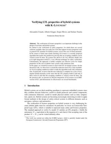
Model Checking LTL Properties with Bounded TracesP1 :int s 0;while ( true ){s 1 - s ;};P2 :int s 0;while ( true ){s 1;s 0;};7P3 :int s 0;s 1;while ( true ){s 0;s 1;};Fig. 2 Programs with identical infinite traces but different behaviour on finiteunwindings for γ G({s 0} F{s 1}).Lamport [33]. We identify a C program P with the set of all traces T (P )that correspond to this Kripke structure, and say that an LTL formula ϕholds for P if ϕ holds for all w T (P ).Note that we use a linear-time rather than a branching-time approachand thus there are no explicit path quantifications (i.e., CTL -style operators A and E). There is, however, an implicit universal quantification overall possible interleavings and program executions.3.2 LTL over Finite TracesThe standard LTL semantics is defined over infinite traces, but as we are using a bounded model checker to analyse the program, we explore only finitetraces. Like other bounded model checkers [11], ESBMC bounds the program executions by limiting the number of times a loop is unrolled, ratherthan limiting the length of traces.2 This guarantees that loop invariants arerespected over the traces. If the program contains at most one potentiallyunbounded loop then the finite traces explored by ESBMC are proper prefixes of the potentially infinite traces of the original program. If the programcontains several potentially unbounded loops then we can still analyse it,using the --partial-loops option. In this case, however, the observed finite traces are not necessarily proper prefixes of the original program traces,and our approach can produce false results, as the symbolic execution cancontinue past unsatisfied loop termination conditions.We use the notation P k to denote the k-fold loop unwinding of the program P . Consider for example the three programs shown in Figure 2 andthe request-response formula γ G({s 0} F{s 1}). Since all threeprograms alternate infinitely often between s 0 and s 1, the single infinite trace produced by each program satisfies γ under the standard LTLsemantics. The situation, however, looks different for the traces producedby finite unwindings (with increasing loop bounds) of the program loops,as the loop structure of the program determines the lengths of the finite2Unstructured goto C code is also handled; every execution of a backward jumpcounts as a “loop iteration” associated with that goto.
8Jeremy Morse, Lucas Cordeiro, Denis Nicole, Bernd Fischerprefixes which are considered. P1 ends with s 1 (i.e., responds to the request) if we unwind the loop an odd number of times, and with s 0 (i.e.,a pending request) otherwise, P2 always ends with s 0, while P3 alwaysends with s 1. P3 is thus intuitively better behaved than both P2 (whichis consistently wrong) and P1 (which behaves erratically). The standard(infinite trace) LTL semantics does not distinguish between the programs.There is a fundamental problem with applying LTL to finite traces. Itis caused by extending the standard interpretation of X as a strong (orexistential) next operator [29] to finite traces, which requires the existenceof a next state to hold. This is counter-intuitive for finite traces, since X trueis now no longer a tautology, as F (i.e., the standard interpretation appliedto finite traces) gives us for all formulas ϕ, [u Xϕ]F if u1 [6].Several approaches tweak the syntax or semantics of LTL to remedy thissituation. Since G and F can be defined relatively straightforwardly on finitetraces, Giannakopolou and Havelund [21] suggested removing X and workwith an X-free subset of LTL. The syntax can instead be extended by addingan additional weak (or universal) next operator X [35], which complementsthe strong next and holds if there is no next state: [u Xϕ]F if u1 .Hence, X true is a tautology. This also gives unwinding laws for F and G,namely Fϕ ϕ XFϕ and Gϕ ϕ XGϕ. Alternatively, the distinctionbetween strong and weak next can be encoded into the semantics ratherthan the syntax, via two different semantic functions which coincide on thetemporal and most Boolean operators, but differ on negation (which flipsbetween both functions) and the atomic propositions, where they reflectthe behaviours of strong and weak next, respectively [19]. Finally, the finitetraces can be systematically extended, e.g., by infinite stuttering of their laststate [33], to allow the use of standard semantics, i.e., defining [u ϕ] [uuωn 1 ϕ]ω for a finite trace u of length n. This is also called the infiniteextension semantics [4], and we say that a BA corresponding to ϕ stutteraccepts u if [u ϕ] .Under the infinite extension semantics, γ (see Figure 2 again) now holdsfor all unwindings of P3 , but not for the unwindings of P2 or P1 . However,in a two valued logic, we cannot distinguish between a formula that (truly)holds because we have seen a good prefix [30] and so all possible continuations of the observed finite trace will be models as well, and one that(presumably) holds because we have not yet seen a bad prefix (i.e., a finitetrace that cannot be prefix of a model) or because it holds if we stutterthe final state infinitely often. In order to realize this distinction, we usea larger truth domain. Bauer et al. [5–7] have proposed and analysed twodifferent domains, B3 { , ?, }, with v ? v , , and ? ?, andB4 { , p , p , }, with v p v p v , , and p p . Under 3 , finite traces are mapped to (resp. ) iff they are good (resp. bad)prefixes; all other finite traces are considered “ugly” and are mapped to theinconclusive truth value ? [5, 7]. In B4 , ? is refined into the two truth values p (“presumably false”) and p (“presumably true”). The interpretationfunction 4 then uses the finite trace semantics with weak next to distin-
Model Checking LTL Properties with Bounded Traces9guish between the two cases (i.e., [u ϕ]4 p iff u is an ugly prefix and[u ϕ]F , and similarly for p ) [6].Our analysis here is based on B4 as well, but we use a different interpretation function from Bauer et al. [6]. In particular, we use the infiniteextension semantics to resolve ugly prefixes into presumably good or presumably bad. The advantage of this approach is that we do not need toresort to the weak-next operator and can define the finite trace semanticsin terms of the standard semantics only. The use of stutter extension in thisway is naturally compatible with the stutter-invariant semantics introducedby Lamport [33] for computer programs but does not require it.Definition 2 The bounded trace semantics of LTL formulas is given by iff w Σ ω · [uw ϕ]ω p iff [uuω ϕ] w Σ ω · [uw ϕ] ωωn 1[u ϕ]B ω p iff [uuω ϕ] w Σ·[uw ϕ] ωω n 1 ω iff w Σ · [uw ϕ]ω for a finite trace u Σ of length n 0 and an LTL formula ϕ.In our case, all program traces are guaranteed to be non-empty, becauseall global variables have defined initial values, which then form the initialstate. We extend the interpretationd to sets of traces by taking the meet overall elements, i.e., [U ϕ]B u U [u ϕ]B . We say that ϕ holds (resp.presumably holds) for a C program P if [T (P ) ϕ]B (resp. p ). Wefinally say ϕ holds (resp. presumably holds) if [Σ ω ϕ]B (resp. p )and define the notion of failing resp. presumably failing correspondingly.The bounded trace semantics is an extension of our earlier work [37]where we only used the infinite stutter semantics. Consequently, we wereeffectively working only with the inconclusive truth values p and p , whilewe add the definitive truth values and here.3.3 LTL Model Checking vs. LTL Runtime VerificationFinite LTL semantics similar to the bounded trace semantics we are usinghere have been developed largely for run-time monitoring and verificationpurposes [34], and due to the focus on finite traces, our approach has somesimilarities with run-time verification, but one key difference remains. Runtime verification only considers actually observed behaviours, one at a time,while we analyse all possible behaviours at the same time. This difference becomes prominent with non-determinism, even for single-threaded programs.Consider for example the program Qint p 0 , q 0; p 1; if (*){ p 0}; if (*){ q 1};where “*”denotes a non-deterministic choice and p and q are zero-initialisedglobal variables. Q can produce four finite traces, depending on the particular non-deterministic choices:
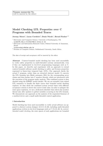
10Jeremy Morse, Lucas Cordeiro, Denis Nicole, Bernd Fischer(i) [{p 0} {q 0}, {p 1} {q 0}],(ii) [{p 0} {q 0}, {p 1} {q 0}, {p 1} {q 1}],(iii) [{p 0} {q 0}, {p 1} {q 0}, {p 0} {q 0}], and(iv) [{p 0} {q 0}, {p 1} {q 0}, {p 0} {q 0}, {p 0} {q 1}].Now consider the LTL formula ψ X({p 1} U {q 1}). Clearly, ψ doesnot hold for the traces (iii) and (iv), and over these, 3 , 4 , and B allmap ψ to . However, in run-time verification, there is no guarantee thatwe ever observe these traces, so the assurance we gain from its results islimited. Our approach, however, will work out that [T (Q) ψ]B andhence Q can fail ψ. Moreover, if we consider Q0 to be the variant of Q whereq is initialised with one, we find [T (Q0 ) ψ]B as well. Finally, if wechange Q to Q00int p 0 , q 0; p 1; if (*){ q 1};then (iii) and (iv) become impossible, and our approach will calculate[T (Q00 ) ψ]B p , meaning that no finite trace produced by Q00 is adefinitive counter-example but, on stuttering, ψ does not hold for all traces.4 Characterizing Program Behaviours Using B4Definition 2 characterises the truth value in B4 of an LTL formula ϕ withrespect to a single finite trace u. In this section we now show how we canuse the Büchi automaton for the never claim to effectively calculate thetruth value of the formula with respect to the finite traces of a programP . In Section 4.1, we briefly recall the basic notions of Büchi automata. InSection 4.2 we characterise the relationship between truth values in B4 andvalidity of never claims over B2 , while we describe the high-level structureof our algorithm in Section 4.3.4.1 Büchi AutomataBüchi automata (BA) are finite-state automata over infinite words firstdescribed by Büchi [8]. We follow Holzmann’s presentation [24] and definea BA as a tuple B (S, s0 , L, T, F ) where S is a finite set of states, s0 Sthe initial state of the BA, L a finite set of labels, T : S L 2S a statetransition function and F S a set of accepting states. A run is a sequenceof state transitions taken by B as it operates over some input. A run isaccepted if B can pass through an accepting state s F infinitely often alongthe run. B may be deterministic or non-deterministic but in the following,we will consider only non-deterministic BAs, since deterministic BAs needa more complicated acceptance condition in order to model LTL. A BA isin reduced form [1] if it has no rejecting traps, i.e., if the BA has a possiblenext state, then there is some extension of the trace that is accepted.
Model Checking LTL Properties with Bounded Tracesinit!{pressed} {charge min}inittrue11true{charge min}!{charge min}&&{pressed}T0 2true2!{charge min}Fig. 3 The left BA accepts the example from the introduction,G({pressed} F{charge min}). The right BA is its negation, used forthe never claim in our monitor.A number of algorithms exist for converting an LTL formula to a BAaccepting a program trace [20, 22, 42]. We use the ltl2ba [20] algorithm andtool. Figure 3 illustrates the BA produced from the example LTL formula inthe introduction. Its labels (i.e., input symbols) are propositions composedfrom the primitive C-expressions used in the LTL formula.4.2 Truth Values in B4 and Standard Validity of Never ClaimsAs noted above, Definition 2 characterises the truth value in B4 of an LTLformula ϕ with respect to a single finite trace u. However, for model checkingϕ over a program P this is not yet suitable. First, we need to express thetruth value in B4 in terms of the validity of the never claim under the twovalued standard semantics. This allows us to use the BA for the never claimdirectly, and avoids the need to define an explicit acceptance criterion forthe four-valued logics. The following lemma addresses this problem. Notethat we do not need a complete characterisation of all truth values in B4 .Lemma 1(i) [u ϕ]B iff @w Σ ω · [uw ϕ]ω (ii) [u ϕ]B w p iff [uuωn 1 ϕ]ω (iii) [u ϕ]B iff w Σ ω · [uw ϕ]ω Proof (i) Since the standard semantics ω (cf. Figure 1) is defined over B2 ,@w Σ ω · [uw ϕ]ω is equivalent to w Σ ω · [uw ϕ]ω ,and thus to w Σ ω · [uw ϕ]ω , which gives us the claim.ω(ii) Similarly, [uuωn 1 ϕ]ω is equivalent to [uun 1 ϕ]ω ,pwhich holds if and only if [u ϕ]B or [u ϕ]B .(iii) This follows directly from the definitions of ω and B .
12Jeremy Morse, Lucas Cordeiro, Denis Nicole, Bernd FischerSecond, the program P may be non-deterministic and produce more thanone trace. We thus need to consider the minimum truth value attained overall of its possible traces T (P ). The following lemma addresses this problem.Lemma 2(i) [U ϕ]B iff @u U, w Σ ω · [uw ϕ]ω (ii) [U ϕ]B w p iff @u U · [uuωn 1 ϕ]ω (iii) [U ϕ]B iff u U · w Σ ω · [uw ϕ]ω dProof Recall that u U [u ϕ]B [U ϕ]B . Then:(i) By Lemma 1 @u U, w Σ ω · [uw ϕ]ω is equivalent to u U · [u ϕ]B ; hence, [U
LTL semantics to handle the nite traces that bounded model checking explores; we thus check the combined system several times with di erent acceptance criteria to derive the correct truth value. In order to mitigate the state space explosion, we use a dedicated scheduler that selects the monitor