Transcription
Server Load PredictionSuthee Chaidaroon (unsuthee@stanford.edu)Joon Yeong Kim (kim64@stanford.edu)Jonghan Seo (jonghan@stanford.edu)AbstractEstimating server load average is one of the methods that can be used to reduce the cost of renting acloud computing service. By making an intelligent guess of how busy a server would be in the nearfuture, we can scale up or down computing requirements based on this information. In this experimentwe have collected website access and server uptime logs from a web application company's websiteand extracted information from these data. We are able to build a prediction model of server loadaverage by applying a linear regression, locally weight linear regression, multinomial logisticregression, and support vector regression. Our experiment shows a trade-off between computingefficiency and prediction accuracy among our selected learning algorithms. The locally weight linearregression has the most accurate prediction of server load average but takes a long time to converge.On the other hand, the support vector regression converges very quickly but performs poorly onsparse training samples. At the end of this paper, we will discuss on improvements we can do forfuture experiments.IntroductionOur clients operate a website and rent the cloud servers of Amazon EC2. The EC2 allows them toscale the computing capacity up and down as they need and they only pay for the computing capacitythat their website actually uses. This task is tedious and can be automated. We think that there shouldbe a way to automatically this task without having clients to monitor their server activities all the time.Our solution is to estimate a server load average based on the website users' activities. We assumethat the number of activities and transactions determines a server load average. We use thisassumption to build a prediction model.MethodologyWe collected website access logs and server uptime logs during the past few months and processedthose two files by merging transactions and load average that occur in the same time interval. Wethen use this processed file as our training samples. Each line of a training sample file has a timeinformation, number of unique IP addresses, the total size of contents, protocol, and the load averageof the last 1, 5, and 15 minutes. Below are parts of access log and uptime files:99.63.73.46 - - [24/Oct/2009:00:00:05 0000] "GET /cgi-bin/uptime.cgi HTTP/1.0" 200 7199.63.73.46 - - [24/Oct/2009:00:01:21 0000] "GET /logs/error log HTTP/1.1" 200 325999.63.73.46 - - [24/Oct/2009:00:01:31 0000] "GET /logs/error log HTTP/1.1" 304 99.63.73.46 - - [24/Oct/2009:00:05:04 0000] "GET /cgi-bin/uptime.cgi HTTP/1.0" 200 7199.63.73.46 - - [24/Oct/2009:00:07:00 0000] "GET /crossdomain.xml HTTP/1.1" 200 20299.63.73.46 - - [24/Oct/2009:00:07:00 0000] "GET /m/s/248/f/1280/f248-1280-6.bpk HTTP/1.1" 200 68099.63.73.46 - - [24/Oct/2009:00:07:00 0000] "GET /m/s/271/f/1301/f271-1301-6.bpk HTTP/1.1" 200 23000Table 1. Part of access log1Mon Oct 12 15:50:02 PDT 2009:: 18:50:02 up 95 days, 27 min, 0 users, load average: 0.23, 0.06, 0.02Mon Oct 12 15:55:01 PDT 2009:: 18:55:02 up 95 days, 32 min, 1 user, load average: 0.00, 0.02, 0.00Mon Oct 12 16:00:02 PDT 2009:: 19:00:03 up 95 days, 37 min, 1 user, load average: 0.00, 0.00, 0.00Mon Oct 12 16:05:06 PDT 2009:: 19:05:07 up 95 days, 42 min, 1 user, load average: 0.00, 0.00, 0.00Mon Oct 12 16:10:01 PDT 2009:: 19:10:02 up 95 days, 47 min, 1 user, load average: 0.53, 0.41, 0.16Mon Oct 12 16:15:01 PDT 2009:: 19:15:02 up 95 days, 52 min, 1 user, load average: 0.05, 0.20, 0.14Table 2. Part of uptime log2
After parsing and processing the data, the features available for us to use are: day of the week(Monday, Tuesday, etc.), month, date, year, hour, minute, second, number of unique users, numberof POST requests, number of GET requests, and content size of the interaction.The diagram below represents our prediction model:At the very bottom level, we predict the server load based on time. The problem of predicting theserver load only based on time would be extremely difficult to solve. So, we decided to divide theproblem into two parts, one to predict the server load, and another, to predict the user features basedon time. For regressions and classifications tests in the following section, we will assume that the userfeatures were correctly predicted.The output value that we tested was chosen to be the 5-minute average server load because theuptime command was run every 5 minutes on the server.Experimental ResultLinear RegressionWe assume that the user features such as number of unique users and number of requests, etc. werecorrectly predicted by h1(t). This assumption had to be made because of amount of data which wasnot sufficient to predict the user features since the logs had been made only since this August. Thefeatures month and year were dropped from the feature lists to create a training matrix that is of fullrank.To create a larger set of features, we concatenated powers of the matrix X to the original matrix. So,our training matrix,2nX [Xorig Xorig . Xorig ].
Since the full rank of matrix X could not be preserved from n 5, we could only test the caseswhere n 1,2,3,4. To come up with the optimal n, some tests were done to compute the averagetraining and test errors. The following graph shows the errors.As we can see from the graph above, the overall error actually got worse as we increased the numberof features used. However, because we thought that n 3 gave a prediction curve of shape closer tothe actual data, we picked n 3. Below are the plots of parts of the actual and predicted server loadfor training and test data. The corresponding errors with respect to n are listed below:naveragetraining erroraverage .07840.3471As the two graphs display, the predictions are not as accurate as it ought to be. However, the trendsin the server load are quite nicely fit. For the above regression, the training error was 0.0652, and thetest error was 0.0683. Since the shape of the curve is quite nicely fit, for our purpose of predicting theserver load to increase or decrease the number of servers, we could amplify the prediction curve by aconstant factor to reduce the latency experienced by the users, or do the opposite to reduce thenumber of operating servers.Multinomial Logistic RegressionIn order to transform our problem into a logistic regression problem, we classified the values of theserver load (CPU usage) into ten values (0,1, , 9) as follows: if the CPU usage was less than orequal to 0.10, it would be 0; else if less than or equal to 0.20, it would be 1; ; else if less than or
equal to 0.90, it would be 8; else it would be 9. We trained 10 separate hypotheses hi for eachclassification. For testing, the system would choose the classification that gives us the highestconfidence level.We use the same approach as linear regression case to find the maximum power of the matrix wewant to use when coming up with the matrix X, where2nX [Xorig Xorig . Xorig ].The following plots for training and test errors were acquired:naverageaverage testtraining 0.03710.0360As in the linear regression case, we chose n 3 for logistic regression. The following is the resultingplot of our prediction compared to the actual data.As we can see, the multinomial logistic regression always outputs 0 as the classification no matterwhat the features are. This is in part because too many of our data points has Y-values of 0 as thebelow histogram shows. Because the company we got the data from has just launched, the serverload is usually very low. As the website becomes more popular, we would be able to obtain a better
result since the Y-values will be more evenly distributed.Locally weight linear regressionLike linear regression, we first assumed all features used as a input, such as number of users, totalnumber of requests and so on, were correctly predicted byfor the same reason. For buildingup a hypothesis, we had to determine what weight function we would use. In common sense, it isreasonable that server loads after five or ten minutes would be dependent on previous several hoursof behavior so we decided to useas a weight function in our hypothesis. However, for using the weight function we were needed to findout the optimal value of which is the bandwidth of the bell-shaped weight function. So we usedHold-out Cross Validation for picking up the optimal and the way and results are as .04240.04270.05940.05940.0620
000.0563First of all, we had picked 70% of the original data randomly and named it as training data and didagain 30% and named testing data. Then we trained the hypothesis with various values ofon thetraining data and applied testing data on the hypotheses and got test errors in each value of . Abovechart shows test errors of sever loads tested on hypothesis h(t,u) with various . Above plot displaysthe pattern of the test errors with respect to . As we can see in the chart and graph, at 0.03, thetest error is the smallest value on all of three cases so we picked up this one for our weight function.Above plots show the actual server load and prediction of test and train data, respectively. As makinga prediction on every unit of query point x is prohibitively time consuming process, the prediction ismade on each query point in train and test data. Though it seems that it followed the pattern of actualload, sometimes it could not follow spikes and it needed very long time to predict even on querypoints of test so it might not be suitable to be used in a real time system which would be needed in ageneral sever load prediction system. Thus, it is desirable that locally weighted regression will betrained just on previous several hours not on whole previous history if sufficient training data weregiven.Support Vector RegressionWe use SVM Light3 to perform a regression. We remove all zero features ( which indicating that aserver is idle ) and select training samples randomly. The trade-off between training error and marginis 0.1 and epsilon width of the tube is 1.0. We use a linear kernel and found that there are 148 support
vectors and the norm of the weight vectors are 0.00083. The training error is 0.479 andthe testing error is 0.319.Above plots are parts of the results from the Support vector regression. The red curve is an actualdata and the blue curve is the prediction. Although the support vector regression is quickly convergedfor 6,000 training data set, its prediction has higher training and testing errors than the rest of learningalgorithms. We tried to adjust an epsilon width and found that the higher epsilon width will only offsetan estimation by a fixed constant.ConclusionThe prediction from the locally weight linear regression yields the smallest testing error but it takes anhour to process 6,000 training samples. The linear regression also yields an acceptable predictionwhen we concatenated the same feature vectors up to a degree of 3. Both Multinomial logisticregression and support vector regression do not perform well with sparse training data. Supportvector regression, however, takes only a few minutes to converge, but yields the largest trainingerror.IssuesBias with sparse dataOur learning algorithms cannot estimate an uptime reliably because there are almost 90% of thetraining samples have an uptime value between 0.0 and 0.1. We believe that the data we havecollected are not diverse due to the low number of activities of our testing web server.Not enough featuresIn our experiment, a dimension of the feature vectors are 10. 7 of them are part of a timestamp. Wethink that we do not have enough data to capture the current physical state of the cloud servers suchas the memory usage, bandwidth, and network latency.weak prediction modelWe think that our decision to use the number of transactions and unique users as part of the featurevectors does not accurately model the computing requirements of the cloud servers. An access logfile and uptime file are generated separately by different servers. Our assumption that a user activityis the only main cause of high server load average may not be accurate. It is possible that a singletransaction could cause a high demand for a computing requirement.Future workWe have found a research paper that describes the use of website access logs to predict a user'sactivities by clustering users based on their recent web activities, we like this idea and think that it ispossible to categorize website users based on their computing demands. When these type of usersare using the website, we think there is a high chance of increasing the computing requirements.References
[1] Access Log specification. http://httpd.apache.org/docs/2.0/logs.html[2] Uptime specification. http://en.wikipedia.org/wiki/Uptime[3] SVMLight. Vers. 6.02. 382K. Aug 14. 2008. Thorsten Joachims. Nov 15. 2009.
Server Load Prediction Suthee Chaidaroon (unsuthee@stanford.edu) Joon Yeong Kim (kim64@stanford.edu) Jonghan Seo (jonghan@stanford.edu) Abstract Estimating server load average is one of the methods that can be used to reduce the cost of renting a cloud computing service. By making an intelligent guess of how busy a server would be in the near