Transcription
Chapter 3Continuous Random Variables3.1IntroductionRather than summing probabilities related to discrete random variables, here forcontinuous random variables, the density curve is integrated to determine probability.Exercise 3.1 (Introduction)Patient’s number of visits, X, and duration of visit, Y .density, pmf f(x)10.75density, pdf f(y) y/6, 2 y 4probability less than 1.5 sum of probabilityat specific valuesP(X 1.5) P(X 0) P(X 1) 0.25 0.50 0.751probability less than 3 area under curve,P(Y 3) 5/122/30.501/2probability at 3,P(Y 3) 0P(X 2) 0.250.251/30120123x4probability (distribution): cdf F(x)110.750.750.50probability less than 1.5 value of functionF(1.5 ) P(X 1.5) 0.750.2501probability value of function,F(3) P(Y 3) 5/120.25201234xFigure 3.1: Comparing discrete and continuous distributions73
74Chapter 3. Continuous Random Variables (LECTURE NOTES 5)1. Number of visits, X is a (i) discrete (ii) continuous random variable,and duration of visit, Y is a (i) discrete (ii) continuous random variable.2. Discrete(a) P (X 2) (i) 0 (ii) 0.25 (iii) 0.50 (iv) 0.75(b) P (X 1.5) P (X 1) F (1) 0.25 0.50 0.75requires (i) summation (ii) integration and is a value of a(i) probability mass function (ii) cumulative distribution functionwhich is a (i) stepwise (ii) smooth increasing functionRP(c) E(X) (i)xf (x) (ii) xf (x) dx(d) V ar(X) (i) E(X 2 ) µ2 (ii) E(Y 2 ) µ2 (e) M (t) (i) E etX (ii) E etY(f) Examples of discrete densities (distributions) include (choose one or more)(i) uniform(ii) geometric(iii) hypergeometric(iv) binomial (Bernoulli)(v) Poisson3. Continuous(a) P (Y 3) (i) 0 (ii) 0.25 (iii) 0.50 (iv) 0.75ix 3R3232225 12 12 12(b) P (Y 3) F (3) 2 x6 dx x12x 2requires (i) summation (ii) integration and is a value of a(i) probability density function (ii) cumulative distribution functionwhich is a (i) stepwise (ii) smooth increasing functionRP(c) E(Y ) (i)yf (y) (ii) yf (y) dy(d) V ar(Y ) (i) E(X 2 ) µ2 (ii) E(Y 2 ) µ2 (e) M (t) (i) E etX (ii) E etY(f) Examples of continuous densities (distributions) include (choose one ormore)(i) uniform(ii) exponential(iii) normal (Gaussian)(iv) Gamma(v) chi-square(vi) student-t(vii) F
Section 2. Definitions (LECTURE NOTES 5)3.275DefinitionsRandom variable X is continuous if probability density function (pdf) f is continuousat all but a finite number of points and possesses the following properties: f (x) 0, for all x,R f (x) dx 1,Rb P (a X b) a f (x) dxThe (cumulative) distribution function (cdf) for random variable X isZ xf (t) dt,F (x) P (X x) and has properties limx F (x) 0, limx F (x) 1, if x1 x2 , then F (x1 ) F (x2 ); that is, F is nondecreasing,Rb P (a X b) P (X b) P (X a) F (b) F (a) a f (x) dx,Rxd F 0 (x) dxf (t) dt f (x). f(x) is positivedensity, f(x)probabilitya)cdf F(a) P(X aprobabilityb) F(b) - F(a)P(a X total area 1xaFigure 3.2: Continuous distributionThe expected value or mean of random variable X is given byZ µ E(X) xf (x) dx, the variance isσ 2 V ar(X) E[(X µ)2 ] E(X 2 ) [E(X)]2 E(X 2 ) µ2b
76Chapter 3. Continuous Random Variables (LECTURE NOTES 5)with associated standard deviation, σ The moment-generating function is σ2. M (t) E etX Z etX f (x) dx for values of t for which this integral exists.Expected value, assuming it exists, of a function u of X isZ E[u(X)] u(x)f (x) dx The (100p)th percentile is a value of X denoted πp whereZ πpf (x) dx F (πp )p and where πp is also called the quantile of order p. The 25th, 50th, 75th percentilesare also called first, second, third quartiles, denoted p1 π0.25 , p2 π0.50 , p3 π0.75where also 50th percentile is called the median and denoted m p2 . The mode is thevalue x where f is maximum.Exercise 4.2 (Definitions)1. Waiting time.Let the time waiting in line, in minutes, be described by the random variableX which has the following pdf, 1x, 2 x 4,6f (x) 0,otherwise.density, pdf f(x)1probability value of function,F(3) P(X 3) 5/12probability less than 3 area under curve,P(X 3) 5/122/31/2probability, cdf F(x)10.75probability at 3,P(X 3) 01/30.2501234x0Figure 3.3: f(x) and F(x)1234x
Section 2. Definitions (LECTURE NOTES 5)77(a) Verify function f (x) satisfies the second property of pdfs, x 4Z Z 4x24222121x dx f (x) dx 12 x 2 12 1212 2 6(i) 0 (ii) 0.15 (iii) 0.5 (iv) 1(b) P (2 X 3) Z32(i) 0 (ii)512(iii)9121x2x dx 6121x6x 23222 12 12(iv) 13212(c) P (X 3) P (3 X 3) (i) True (ii) FalseSo the pdf f (x) x 3 3212 0 6 f (3) 16· 3 0.5determined at some value of x does not determine probability.(d) P (2 X 3) P (2 X 3) P (2 X 3) P (2 X 3)(i) True(ii) Falsebecause P (X 3) 0 and P (X 2) 0(e) P (0 X 3) Z32x21x dx 612 x 3 3222 12 12 3222 12 12x 259(iii) 12(iv) 112Why integrate from 2 to 3 and not 0 to 3?(i) 0 (ii)(f) P (X 3) Z2(i) 0 (ii)512(iii)91231x2x dx 6122(i) 0 (ii)(iii)912x 2(iv) 1(g) Determine cdf (not pdf) F (3).ZF (3) P (X 3) 512 x 331x2x dx 612 x 3x 22232 12 12(iv) 1(h) Determine F (3) F (2).ZF (3) F (2) P (X 3) P (X 2) P (2 X 3) 231x2x dx 61259(iii) 12(iv) 112because everything left of (below) 3 subtract everything left of 2 equals what is between 2 and 3(i) 0 (ii) x 3 x 232 22 12 12
78Chapter 3. Continuous Random Variables (LECTURE NOTES 5)(i) The general distribution function (cdf) is Rx R 0 dt 0,it xx tt2F (x) dt 12 62 t 2 1,2x 2,x2124,12 2 x 4,x 4.24In other words, F (x) x12 12 x 12 4 on (2, 4]. Both pdf density and cdfdistribution are given in the figure above.(i) True (ii) False(j) F (2) 2212 412 (i) 0 (ii)512(iii)912(iv) 1.(k) F (3) 32 412 (i) 0 (ii)512(iii)912(iv) 1.12 (m) P (X 3.5) 1 P (X 3.5) 1 F (3.5) 1 (i) 0.3125 (ii) 0.4425 (iii) 0.7650 (iv) 1. (l) P (2.5 X 3.5) F (3.5) F (2.5) (i) 0 (ii) 0.25 (iii) 0.50 (iv) 1.3.5212 412 2.52123.5212 412412 (n) Expected value. The average wait time isZ 4Zxxf (x) dx µ E(X) 21x6 4Zdx 2x2x3dx 618 4243 23 18 1823(ii) 28(iii) 31(iv) 35.9999library(MASS) # INSTALL once, RUN once (per session) library MASSmean - 4 3/18 - 2 3/18; mean; fractions(mean) # turn decimal to fraction(i)[1] 3.111111[1] 28/9(o) Expected value of function u x2 .E X2 Z 2 Zx f (x) dx 4x2 21x6 Z4dx 2x3x4dx 624(i) 9 (ii) 10 (iii) 11 (iv) 12.(p) Variance, method 1. Variance in wait time is2σ V ar(X) E X2 2 µ 10 289 2232635(ii) 81(iii) 31(iv) 81.8181library(MASS) # INSTALL once, RUN once (per session) library MASSsigma2 - 10 - (28/9) 2 ; fractions(sigma2) # turn decimal to fraction(i) 4 244 24 24 24
Section 2. Definitions (LECTURE NOTES 5)79[1] 26/81(q) Variance, method 2. Variance in wait time isZ 22σ V ar(X) E[(X µ) ] (x µ)2 f (x) dx 4 2 281 x x dx962 Z 4 3x56x2 784x dx6544862 4x4 56x3 784x2 24162972 2Z232635(ii) 81(iii) 31(iv) 81.8181library(MASS) # INSTALL once, RUN once (per session) library MASSsigma2 - (4 4/24 - 56*4 3/162 784*4 2/972) - (2 4/24 - 56*2 3/162 784*2 2/972)fractions(sigma2) # turn decimal to fraction(i)[1] 26/81(r) Standard deviation. Standard deviation in time spent on the call is,r 26 σ σ2 81(i) 0.57 (ii) 0.61 (iii) 0.67 (iv) 0.73.(s) Moment generating function.Z tXM (t) E[e ] etx f (x) dx Z 41tx ex dx62Z1 4 tx xe dx6 2 41 tx x1 e 26tt x 2 1 4t 411 2t 21 e e ,6t t26t t2t 6 0.(i) True (ii) Falseuse integration by parts for t 6 0 case:Ru dv uv Rv du where u x, dv etx dx.
80Chapter 3. Continuous Random Variables (LECTURE NOTES 5)(t) Median. Since the distribution function F (x) π0.50 occurs whenF (m) P (X m) sorm π0.50 x2 4,12then median m 1m2 4 12212 4 2(i) 1.16 (ii) 2.16 (iii) 3.16negative answer m 3.16 is not in 2 x 4, so m 6 3.162. Density with unknown a. Find a such that 2ax , 1 x 5,f (x) 0,otherwise.density, pdf f(x)1probability, cdf F(x) P(X x)10.750.750.500.500.250.25012345x012345 xFigure 3.4: f(x) and F(x)(a) Find constant a. Since the cdf F (5) 1, andZF (x) 1xt3at dt a32then t x t 1ax3 aa(x3 1) 333a(53 1)124a 1,331(iii) 124F (5) so a (i)3124(ii)2124(b) Determine pdf.f (x) ax2 (i)3x2124(ii)2x2124(iii)1x2124
Section 2. Definitions (LECTURE NOTES 5)81(c) Determine cdf.F (x) (i)3(x3124 1) (ii)a(x3 1)3x3 1 312432(x3124 1) (iii)1(x3124 1)(d) Determine P (X 2).1 3(2 1) 124P (X 2) 1 P (X 2) 1 F (2) 1 (i)61124(ii)117124(iii)61117(e) Determine P (X 4).1 3(4 1) 124P (X 4) 1 P (X 4) 1 F (4) 1 (i)61124(ii)117124(iii)61117(f) Determine P (X 4 X 2).P (X 4 X 2) (i)116124(ii)117124(iii)P (X 4)61/124P (X 4 X 2) P (X 2)P (X 2)117/12461117(g) Expected value.ZZ xf (x) dx µ E(X) (i)11431(ii)115315 x1(iii)11631(iv)3 2x124 Zdx 153x33x4dx 124496117.312 5 13 · 54 3 · 14 496496(h) Expected value of function u x . 5Z Z 5 Z 5 43 23x3x53 · 55 3 · 15222E(X ) x f (x) dx xxdx dx 124620 1620620 11 124(i) 15.12 (ii) 16.12 (iii) 17.12 (iv) 18.12.(i) Determine 25th percentile (first quartile), p1 π0.25 .Since F (x) 1(x3124 1), then,F (π0.25 ) 113(π0.25 1) 0.25 ,1244and sorπ0.25 3124 1 4(i) 2.38 (ii) 3.17 (iii) 4.17The π0.25 is that value where 25% of probability is at or below (to the left of) this value.
82Chapter 3. Continuous Random Variables (LECTURE NOTES 5)(j) Determine π0.01 .F (π0.01 ) and soπ0.01 13 1) 0.01,(π0.01124 30.01 · 124 1 (i) 1.31 (ii) 3.17 (iii) 4.17The π0.01 is that value where 1% of probability is at or below (to the left of) this value.3. Piecewise pdf. Let random variable X have pdf 0 x 1, x,2 x, 1 x 2,f (x) 0,elsewhere.density, pdf f(x)probability, cdf F(x) P(X x)110.750.750.500.500.250.2501x20123xFigure 3.5: f(x) and F(x)(a) Expected value.Z µ E(X) xf (x) dx Z 1Z2x (x) dx x (2 x) dx01Z 1Z 2 2 x dx 2x x2 dx01 2 3 1 2x2xx3 3 023 1 3 310231322 2 1 3333 (i) 1 (ii) 2 (iii) 3 (iv) 4.
Section 2. Definitions (LECTURE NOTES 5)83(b) E (X 2 ).E X(i)46(ii)2 Z1Z2x2 (2 x) dxx (x) dx Z 2 1Z0 1 2x2 x3 dxx3 dx 10 4 1 3 2xx42x 4 034 1 4 4012(2)3 242(1)3 14 443434 66256(iii)(iv) 76 .14 7σ 2 Var(X) E X 2 µ2 12 611(iii) 5 (iv) 6 .(c) Variance.(i)13(ii)(d) Standard deviation. σ rσ2 1 6(i) 0.27 (ii) 0.31 (iii) 0.41 (iv) 0.53.(e) Median. Since the distribution function is 0 ix R2 x t dt t2 x2 ,20t 0ixF (x) Rxt2 (2 t) dt F (1) 2t 2 1 t 1 1,F (1) 1,2so add12x 00 x 1,12 2x x22 (2(1) to F (x) for 1 x 2then median m occurs when m2 2 12 ,2F (x) 2m m2 1 12 , 1,0 x 1,1 x 2,x 2.so for both 0 x 1 and 1 x 2, m (i) 1 (ii) 1.5 (iii) 212)2 12 ,1 x 2,x 2.
843.3Chapter 3. Continuous Random Variables (LECTURE NOTES 5)The Uniform and Exponential DistributionsTwo special probability density functions are discussed: uniform and exponential.The continuous uniform (rectangular) distribution of random variable X has density 1, a x b,b af (x) 0,elsewhere,where “X is U (a, b)” means “X is uniform over [a,b]”, distribution function, x a, 0x aa x b,F (x) b a1x b,and its expected value (mean), variance and standard deviation are,a bµ E(X) ,2(b a)2σ V ar(X) ,122σ pV ar(X),and moment-generating function is etb etaM (t) E etX , t 6 0.t(b a)The continuous exponential random variable X has density λxλe , x 0,f (x) 0,elsewhere,distribution function, F (x) 01 e λxx 0,x 0,and its expected value (mean), variance and standard deviation are,µ E(X) 1,λσ 2 V (Y ) 1,λ2σ 1,λand moment-generating function is M (t) E etX Notice if θ 1λλ,λ tt λ.in the exponential distribution,1 xf (x) e θ ,θxF (x) 1 e θ ,µ σ θ,M (t) Exercise 3.3 (The Uniform and Exponential Distributions)θ.1 tθ
Section 3. The Uniform and Exponential Distributions (LECTURE NOTES 5)851. Uniform: potato weights. An automated process fills one bag after anotherwith Idaho potatoes. Although each filled bag should weigh 50 pounds, in fact,because of the differing shapes and weights of each potato, each bag weight, X,is anywhere from 49 pounds to 51 pounds, with uniform density: 0.5, 49 x 51,f (x) 0,elsewhere.(a) Since a 49 and b 51, the distribution is x 49, 0x 4949 x 51,F (x) 51 491x 52,and so graphs of density and distribution are given in the figure.(i) True(ii) Falsedensity, pdf f(x)1probability, cdf F(x) P(X x)10.750.750.500.500.250.250495051x0495051xFigure 3.6: Distribution function: continuous uniform(b) Determine P (49.5 X 51) by integrating pdf.Z 511x i5151 49.51.5P (49.5 X 51) dx 2 x 49.522249.5 2(i) 0.25 (ii) 0.50 (iii) 0.75 (iv) 1.(c) Determine P (49.5 X 51) using cdf.P (49.5 X 51) F (51) F (49.5) 51 49 49.5 49 51 4951 49(i) 0.25 (ii) 0.50 (iii) 0.75 (iv) 1.1 - punif(49.5,49,51) # uniform P(49.5 X 51) 1 - P(X 49.5), 49 x 51[1] 0.75
86Chapter 3. Continuous Random Variables (LECTURE NOTES 5)(d) The chance the bags weight more than 49.5P (X 49.5) 1 P (X 49.5) 1 F (49.5) 1 49.5 49 51 49(i) 0.25 (ii) 0.50 (iii) 0.75 (iv) 1.1 - punif(49.5,49,51) # uniform P(X 49.5) 1 - P(X 49.5), 49 x 51[1] 0.75(e) What is the mean weight of a bag of potatoes?µ E(X) a b49 51 22(i) 49 (ii) 50 (iii) 51 (iv) 52.(f) What is the standard deviation in the weight of a bag of potatoes?ss2(b a)(51 49)2 σ 1212(i) 0.44 (ii) 0.51 (iii) 0.55 (iv) 0.58.(g) Determine probability within 1 standard deviation of mean.P (µ σ X µ σ) P (50 0.58 X 50 0.58) P (49.42 X 50.58)Z 50.581x i50.58 dx 2 x 49.4249.42 2(i) 0.44 (ii) 0.51 (iii) 0.55 (iv) 0.58.(h) Function of X. If it costs 0.0556 (5.56 cents) per pound of potatoes,then the cost of X pounds of potatoes is Y 0.0556X. Determine theprobability a bag of potatoes chosen at random costs at least 2.78.Z 511x i51P (Y 2.78) P (0.0556X 2.78) P (X 50) dx 2 x 5050 2(i) 0.25 (ii) 0.50 (iii) 0.75 (iv) 1.2. Exponential: atomic decay. Assume atomic time-to-decay obeys exponentialpdf with (inverse) mean rate of decay λ 3, 3x3e , x 0,f (x) 0,otherwise.
Section 3. The Uniform and Exponential Distributions (LECTURE NOTES 5)density, pdf f(x)4probability, cdf F(x) P(X x)433221101872345x012345xFigure 3.7: f(x) and F(x)(a) Find F (x). By substituting u 3x, then du 3 dx and soZZZ 3x 3xF (x) 3edx e ( 3) dx eu du eu (i) e 3x (ii) e 3x (iii) 3e 3xthen t x F (x) e 3t t 0 e 3x ( e 3(0) ) (i) e 3x 1 (ii) e 3x 1 (iii) 1 e 3x(b) Chance atomic decay takes at least 2 microseconds, P (X 2), is P (X 2) 1 P (X 2) 1 F (2) 1 1 e 3(2) (i) 0.002 (ii) 0.003 (iii) 0.0041 - pexp(2,3) # exponential P(X 2), lambda 3[1] 0.002478752(c) Chance atomic decay is between 1.13 and 1.62 microseconds isP (1.13 X 1.62) F (1.62) F (1.13) 1 e (3)(1.62) 1 e (3)(1.13) e (3)(1.13) e (3)(1.62) (i) 0.014 (ii) 0.026 (iii) 0.034 (iv) 0.054.pexp(1.62,3) - pexp(1.13,3) # exponential P(1.13 X 1.62), lambda 3[1] 0.02595819(d) Calculate probability atomic rate between mean and 1 standard deviation
88Chapter 3. Continuous Random Variables (LECTURE NOTES 5)below mean. Since λ 3, so µ σ 31 , so 11 1 X P (µ σ X µ) P3 33 1 P 0 X 3 1 F (0) F3 1 1 e (3) 3 1 e (3)(0) (i) 0.33 (ii) 0.43 (iii) 0.53 (iv) 0.63.(e) Check if f (x) is a pdf.Z bZ x b 3x3e 3x dx lim e 3x x 0 lim e 3b ( ex(0) ) 13edx limb 0b 0b or, equivalently,lim F (b) lim 1 e 3b 1b (i) Trueb (ii) False0(f) Show F (x) f (x).F 0 (x) ddF (x) 1 e 3x dxdx(i) 3e 3x (ii) e 3x 1 (iii) 1 e 3xλ(g) Determine µ using mgf. Since M (t) λ t, dλλ0M (t) ,dt λ t(λ t)2so µ M 0 (0) (i) λ (ii) 1 (iii) 1 λ (iv)use quotient rule, since f uv λ,λ tf0 0vu uvv20 1.λ(λ t)(0) λ( 1)(λ t)2 λ(λ t)2 1λif t 0(h) Memoryless property of exponential. Chance atomic decay lasts at least 10microseconds isP (X 10) 1 F (10) 1 (1 e 3(10) ) (i) e 10 (ii) e 20 (iii) e 30 (iv) e 40 .and chance atomic decay lasts at least 15 microseconds, given ithas already lasted at least 5 microseconds isP (X 15 X 5) P (X 15, Y 5)P (X 15)1 (1 e 3(15) ) P (X 5)P (X 5)1 (1 e 3(5) )
Section 3. The Uniform and Exponential Distributions (LECTURE NOTES 5)89(i) e 10 (ii) e 20 (iii) e 30 (iv) e 40 .so, in other words,P (X 15 X 5) P (X 10 5)P (X 15) P (X 10)P (X 5)P (X 5)orP (X 10 5) P (X 10) · P (X 5)This is an example of the “memoryless” property of the exponential, it implies time intervals areindependent of one another. Chance of decay after 15 microsecond, given decay after 5 microseconds,same as chance of decay after 10 seconds; it is as though first 5 microseconds “forgotten”.3. Verifying if experimental decay is exponential. In an atomic decay study, letrandom variable X be time-to-decay where x 0. The relative frequencydistribution table and histogram for a sample of 20 atomic decays (measuredin microseconds) from this study are given below. Does this data follow anexponential distribution?0.60, 0.07, 0.66, 0.17, 0.06, 0.14, 0.15, 0.19, 0.07, 0.360.85, 0.44, 0.71, 1.02, 0.07, 0.21, 0.16, 0.16, 0.01, 0.880.40relative frequency0.35exponential density curve, pdf, f(x)0.300.250.20relative frequencyhistogram approximatesdensity curve0.150.100.05000.20.40.60.81.01.2time-to-decay (microseconds), xFigure 3.8: Histogram of exponential decay times
90Chapter 3. Continuous Random Variables (LECTURE NOTES .8,1](1,1.2]1122221relative exponentialfrequency probability11 (a) Sample mean time-to-decay.x̄ 0.60 0.07 · · · 0.88 20(i) 0.330 (ii) 0.349 (iii) 0.532 (iv) 0.631.x - 8)mean(x)[1] 0.349(b) Approximate λ for exponential. Since approximate mean time-to-decay isµ x̄ 0.349,then, if time-to-decay is exponential, approximate value of λ parameter,since µ λ1 , is11λ µx̄(i) 2.9 (ii) 3.0 (iii) 3.1 (iv) 3.2and so possible model of data might be exponential density(i) 2.9e 3x (ii) 3e 2.9x (iii) 2.9e 2.9x (iv) 3e 3x .(c) Approximate probabilities.Z0.2P (0 X 0.2) 2.9e 2.9x dx 0(i) 0.44 (ii) 0.25 (iii) 0.14 (iv) 0.08.remaining probabilities in table calculated in a similar waypexp(0.2,2.9) - pexp(0,2.9) # exponential P(0 X 0.2), lambda approx 2.9[1] 0.4401016(d) Since sample relative frequencies do not closely match exponential withλ 2.9 in table, this distribution (i) is (ii) is not a good fit to the data.
Section 4. The Normal Distribution (LECTURE NOTES 5)3.491The Normal DistributionThe continuous normal distribution of random variable X, defined on the interval( , ), has pdf with parameters µ and σ, that is, “X is N (µ, σ 2 )”,21f (x) e (1/2)[(x µ)/σ] ,σ 2πand cdfZx21 e (1/2)[(t µ)/σ] dt, σ 2πand its expected value (mean), variance and standard deviation are,pE(X) µ, V ar(X) σ 2 , σ V ar(X),F (x) P (X x) and mgf is σ 2 t2M (t) exp µt .2A normal random variable, X, may be transformed to a standard normal, Z,12f (z) e z /2 ,2πwhere “Z is N (0, 1)” andZzΦ(z) P (Z z) where µ 0, σ 1 and M (t) et2 /212 e t /2 dt,2πusing the following equation,Z X µ.σThe distribution of this density does not have a closed–form expression and so must be solved using numericalintegration methods. We will use both R and the tables to obtain approximate numerical answers.Exercise 3.4 (The Normal Distribution)1. Nonstandard normal: IQ scores.It has been found that IQ scores, Y , can be distributed by a normal distribution.Densities of IQ scores for 16 year olds, X1 , and 20 year olds, X2 , are given by21 e (1/2)[(y 100)/16] ,16 2π21 e (1/2)[(y 120)/20] .f (x2 ) 20 2πf (x1 ) A graph of these two densities is given in the figure.
92Chapter 3. Continuous Random Variables (LECTURE NOTES 5)f(x)16 year old IQsσ 16f(x)20 year old IQsσ 20µ 100µ 120xFigure 3.9: Normal distributions: IQ scores(a) Mean IQ score for 20 year olds isµ (i) 100 (ii) 120 (iii) 124 (iv) 136.(b) Average (or mean) IQ scores for 16 year olds isµ (i) 100 (ii) 120 (iii) 124 (iv) 136.(c) Standard deviation in IQ scores for 20 year oldsσ (i) 16 (ii) 20 (iii) 24 (iv) 36.(d) Standard deviation in IQ scores for 16 year olds isσ (i) 16 (ii) 20 (iii) 24 (iv) 36.(e) Normal density for 20 year old IQ scores is(i) broader than normal density for 16 year old IQ scores.(ii) as wide as normal density for 16 year old IQ scores.(iii) narrower than normal density for 16 year old IQ scores.(f) Normal density for the 20 year old IQ scores is(i) shorter than normal density for 16 year old IQ scores.(ii) as tall as normal density for 16 year old IQ scores.(iii) taller than normal density for 16 year old IQ scores.(g) Total area (probability) under normal density for 20’s IQ scores is(i) smaller than area under normal density for 16’s IQ scores.(ii) the same as area under normal density for 16’s IQ scores.(iii) larger than area under normal density for 16’s IQ scores.(h) Number of different normal densities:(i) one (ii) two (iii) three (iv) infinity.2. Percentages: IQ scores.Densities of IQ scores for 16 year olds, X1 , and 20 year olds, X2 , are given by21 e (1/2)[(y 100)/16] ,16 2π21 e (1/2)[(y 120)/20] .f (x2 ) 20 2πf (x1 )
Section 4. The Normal Distribution (LECTURE NOTES 5)f(x)P(X 84) ?84N(100,162 )P(96 X 120) x100?f(x)96(a)P(X 84) 84?f(x)120(c)932N(100,16 )100x120(b)P(96 X 120) 2?f(x)2N(120,20 )N(120,20 )x96120x(d)Figure 3.10: Normal probabilities: IQ scores(a) For the sixteen year old normal distribution, where µ 100 and σ 16,Z 21 e (1/2)[(y 100)/16] dx1 P (X1 84) 84 16 2π(i) 0.4931 (ii) 0.9641 (iii) 0.8413 (iv) 0.3849.1 - pnorm(84,100,16) # normal P(X 84), mean 100, SD 16[1] 0.8413447(b) For sixteen year old normal distribution, where µ 100 and σ 16,P (96 X1 120) (i) 0.4931 (ii) 0.9641 (iii) 0.8413 (iv) 0.3849.pnorm(120,100,16) - pnorm(96,100,16) # normal P(96 X 120), mean 100, SD 16[1] 0.4930566(c) For twenty year old, where µ 120 and σ 20,P (X2 84) (i) 0.4931 (ii) 0.9641 (iii) 0.8413 (iv) 0.3849.1 - pnorm(84,120,20) # normal P(X 84), mean 120, SD 20[1] 0.9640697(d) For twenty year old, where µ 120 and σ 20,P (96 X2 120) (i) 0.4931 (ii) 0.9641 (iii) 0.8413 (iv) 0.3849.pnorm(120,120,20) - pnorm(96,120,20) # normal P(96 X 120), mean 120, SD 20[1] 0.3849303
94Chapter 3. Continuous Random Variables (LECTURE NOTES 5)(e) Empirical Rule (68-95-99.7 rule). If X is N (120, 202 ), find probabilitywithin 1, 2 and 3 SDs of mean.P (µ σ X µ σ) P (120 20 X 120 20) P (100 X 140) (i) 0.683 (ii) 0.954 (iii) 0.997 (iv) 1.P (µ 2σ X µ 2σ) P (80 X 160) (i) 0.683 (ii) 0.954 (iii) 0.997 (iv) 1.P (µ 3σ X µ 3σ) P (60 X 180) (i) 0.683 (ii) 0.954 (iii) 0.997 (iv) 1.Empirical rule is true for all X which are N (µ, σ 2 ).pnorm(140,120,20) - pnorm(100,120,20);[1] 0.6826895[1] 0.9544997pnorm(160,120,20) - pnorm(80,120,20); pnorm(180,120,20) - pnorm(60,120,20)[1] 0.99730023. Standard normal.Normal densities of IQ scores for 16 year olds, X1 , and 20 year olds, X2 ,21 e (1/2)[(y 100)/16] ,16 2π21 e (1/2)[(y 120)/20] .f (x2 ) 20 2πf (x1 ) Both densities may be transformed to a standard normal with µ 0 and σ 1using the following equation,Z Y µ.σ(a) Since µ 100 and σ 16, a 16 year old who has an IQ of 132 isz 132 100 (i) 0 (ii) 1 (iii) 2 (iv) 316standard deviations above the mean IQ, µ 100.(b) A 16 year old who has an IQ of 84 isz 84 100 (i) 2 (ii) 1 (iii) 0 (iv) 116standard deviations below the mean IQ, µ 100.(c) Since µ 120 and σ 20, a 20 year old who has an IQ of 180 is (i) 0 (ii) 1 (iii) 2 (iv) 3z 180 12020standard deviations above the mean IQ, µ 120.(d) A 20 year old who has an IQ of 100 isz 100 120 (i) 3 (ii) 2 (iii) 1 (iv) 020standard deviations below the mean IQ, µ 120.
Section 4. The Normal Distribution (LECTURE NOTES 5)9516 year oldsmean 100, SD 1652 68 84-3 -2 -1100 116 132 14801 23X, nonstandardZ, standard11020 year oldsmean 120, SD 2060-380-2100-11200140116021803X, nonstandardZ, standardFigure 3.11: Standard normal and (nonstandard) normal(e) Although both the 20 year old and 16 year old scored the same, 110, onan IQ test, the 16 year old is clearly brighter relative to his/her age groupthan is the 20 year old relative his/her age group becausez1 110 120110 100 0.625 z2 0.5.1620(i) True (ii) False(f) The probability a 20 year old has an IQ greater than 90 is 90 120P (X2 90) P Z2 P (Z2 1.5) 20(i) 0.93 (ii) 0.95 (iii) 0.97 (iv) 0.99.1 - pnorm(90,120,20) # normal P(X 90), mean 120, SD 201 - pnorm(-1.5) # standard normal P(Z -1.5), defaults to mean 0, SD 1[1] 0.9331928Or, using Table C.1 from the text,P (Z2 1.5) 1 Φ( 1.5) 1 0.0668 (i) 0.93 (ii) 0.95 (iii) 0.97 (iv) 0.99.Table C.1 can only used on standard normal questions, where Z is N (0, 1).(g) The probability a 20 year old has an IQ between 125 and 135 is 125 120135 120P (125 X2 135) P Z2 P (0.25 Z2 0.75) 2020(i) 0.13 (ii) 0.17 (iii) 0.27 (iv) 0.31.
96Chapter 3. Continuous Random Variables (LECTURE NOTES 5)pnorm(135,120,20) - pnorm(125,120,20) # normal P(125 X 135), mean 120, SD 20pnorm(0.75) - pnorm(0.25) # standard normal P(0.25 Z 0.75)[1] 0.1746663Or, using Table C.1 from the text,P (0.25 Z2 0.75) Φ(0.75) Φ(0.25) 0.7734 0.5987 (i) 0.13 (ii) 0.17 (iii) 0.27 (iv) 0.31.(h) If a normal random variable X with mean µ and standard deviation σcan be transformed to a standard one Z with mean µ 0 and standarddeviation σ 1 usingX µ,Z σthen Z can be transformed to X usingX µ σZ.(i) True (ii) False(i) A 16 year old who has an IQ which is three (3) standards above the meanIQ has an IQ of x1 100 3(16) (i) 116 (ii) 125 (iii) 132 (iv) 148.(j) A 20 year old who has an IQ which is two (2) standards below the meanIQ has an IQ of x2 120 2(20) (i) 60 (ii) 80 (iii) 100 (iv) 110.(k) A 20 year old who has an IQ which is 1.5 standards below the mean IQhas an IQ of x2 120 1.5(20) (i) 60 (ii) 80 (iii) 90 (iv) 95.(l) The probability a 20 year old has an IQ greater than one (1) standarddeviation above the mean isP (Z2 1) P (X2 120 1(20)) P (X2 140) (i) 0.11 (ii) 0.13 (iii) 0.16 (iv) 0.18.1 - pnorm(1) # standard normal P(Z 1), defaults to mean 0, SD 11 - pnorm(140,120,20) # normal P(X 140), mean 120, SD 20[1] 0.1586553(m) Percentile. Determine 1st percentile, π0.01 , when X is N (120, 202 ).Z π0.0121 e (1/2)[(y 120)/20] 0.01,F (π0.01 ) 20 2π and so π0.01 (i) 72.47 (ii) 73.47 (iii) 75.47
Section 5. Functions of Continuous Random Variables (LECTURE NOTES 5)97qnorm(0.01,120,20) # normal 1st percentile, mean 120, SD 20[1] 73.47304Or, using Table C.1 “backwards”, F (π0.01 ) 0.01 whenZ (i) 2.33 (ii) 2.34 (iii) 2.35but since X is N (120, 202 ), 1st percentileπ0.01 X µ σZ 120 20( 2.33) (i) 73.4 (ii) 74.1 (iii) 75.2The π0.01 is that value where 1% of probability is at or below (to the left of) this value.3.5Functions of Continuous Random VariablesAssuming cdf F (x) is strictly increasing (as opposed to just monotonically increasing)on a x b, one method to determine the pdf of a function, Y U (X), ofrandom variable X, requires first determining the cdf of X, F (x), then using F (X)to determine the cdf of Y , F (Y ), and finally differentiating the result,f (y) F 0 (x) dF.duThe second fundamental theorem of calculus is sometimes used in this method,ddyZu2 (y)fX (x) dx fX (u2 (y))u1 (y)du2du1 fX (u1 (y)).dydyRelated to this is an algorithm for sampling at random values from a random variableX with a desired distribution by using the uniform distribution: determine cdf of X, F (x), desired distribution find F 1 (y): set F (x) y, solve for x F 1 (y) generate values y1 , y2 , . . . , yn from Y , assumed to be U (0, 1), use x F 1 (y) to simulate observed x1 , x2 , . . . , xn , from desired distribution.Exercise 3.5 (Functions of Continuous Random Variables)
98Chapter 3. Continuous Random Variables (LECTURE NOTES 5)probability, cdf F(y) P(Y y) y/2 - y 2/16probability, cdf F(x) P(X x) x - x 2/4110.750.750.500.500.250.251023x401234y 2xprobability, cdf F(y) P(Y y) y1/2- y/42probability, cdf F(y) P(Y y) (4 4y y )/16110.750.750.500.500.250.25-1-20121/2y 2 - 2x01234y xFigure 3.12: Distributions of various functions of Y U (X)1. Determine pdf of Y U (X), given pdf of X. Consider density 1 x2 , 0 x 2fX (x) 0elsewhere(a) Calculate pdf of Y 2X, version 1. t xx2tt21 dt t x ,24 t 040 y yP (Y y) P (2X y) P X FX22 y 22yy y 2 ,242 16dFFY0 (y) dyZFX (x) FY (y) fY (y) (i)32 2y32(ii)12x 2y32(iii)12 y32(iv)12 y8 ,where since y 2x, 0 x 2 implies 0 y2 2, or(i) 1 y 2 (ii) 2 y 1 (iii) 0 y 3 (iv) 0 y 4
Section 5. Functions of Continuous Random Variables (LECTURE NOTES 5)99(b) Calculate pdf of Y 2X, version 2. y FY (y) P (Y y) P (2X y) P X 2Z y y 2fX (x) dx FX20 Z y y d y 2dy/21fY (y) fX (x) dx fX 0 1 · dy 02 dy 222y3 2y(ii) 12 2y(iii) 12 32(iv) 21 y8 ,23232Second fundamental theorem of calculus used here, notice cdf of FX (x) is not explicitly calculated.(i)(c) Calculate pdf for Y 2 2X. 2 yFY (y) P (Y y) P (2 2X y) P X 2Z 2 fX (x) dx,2 y2dfY (y) dy2Z 2 y2 1 (i)32 2y32(ii)12 2y32fX (x) dx 0 fX2 y2!·2(iii)12 2 y2 ddy 2 y2 1 2y32(iv)14 y8 ,where since y 2 2x, 0 x 2 implies 0 2 y 2, or2(i) 1 y
74 Chapter 3. Continuous Random Variables (LECTURE NOTES 5) 1.Number of visits, Xis a (i) discrete (ii) continuous random variable, and duration of visit, Y is a (i) discrete (ii) continuous random variable.