Transcription
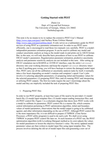
Getting Started with PESTZhulu LinDept. of Crop and Soil SciencesThe University of Georgia, Athens, GA 30602linzhulu@uga.eduThis note is by no means to try to replace the extensive PEST User’s Manual(http://www.sspa.com/pest/) and Surface Water Utilities Manual(http://www.sspa.com/pest/utilities.html). It only serves as a rudimentary guide for PESTnovices of using PEST as a parameter estimation tool. In order to use PEST moreefficiently, one is encouraged to read those two manuals very carefully. PEST is a modelindependent parameter estimation program. It can be used to calibrate any model andconduct uncertainty analysis as long as the model reads in and prints out in ASCII format.But, in this note, we will only describe basic procedures of how to use PEST to calibrateSWAT model’s parameters. Regularization parameter estimation, predictive uncertaintyanalysis and parameter sensitivity analysis are not included in this note. After setting upSWAT simulation run in BASINS or AVSWAT interface, copy the entire txtinoutdirectory into your working directory and keep the original txtinout directory intactso that if anything goes wrong, you will have backups to restore the damaged model inputfiles. PEST carry out all the calibration or uncertainty analysis tasks by itself, it normallytakes a few hours depending on model’s runtime and computer’s speed. User’s jobsinvolve (1) selecting adjustable parameters; (2) preparing initial and boundary values forthe selected parameters; (3) preparing PEST files; and (4) running PEST and interpretingor utilizing PEST outputs. The first two tasks require the user’s knowledge about themodel and they are implicitly included the task of preparing PEST files.1. Preparing PEST filesIn order to run PEST properly, at least four types of file need to be provided: (1) modelbatch file; (2) model input template files; (3) model output reading instruction files; and(4) PEST control file. Figure 1 is a schematic diagram that shows how PEST works witha model to calibrate its parameters. PEST control file is a master file, which containscentral information pertaining to PEST optimization algorithm, initial and boundaryvalues of model parameters, observations that the model output is going to be calibratedagainst, and other information depending on the use of PEST. Although PEST control fileis the most importance file, it is not difficult to prepare if TSPROC (Time SeriesProcessor, a PEST utility program) is used to do such a job. We shall cover usingTSPROC to prepare PEST control file later on. At each iteration of a PEST run, the PESToptimization algorithm (with Levenberg-Marquart method as its core) adjusts the valuesfor model parameters to lessen the objective function’s value. The newly updated modelparameter values are then written to model input files using input template files. Theprocess involves deleting the old set of model input files and generating a new set of1
model input files using the input template files. Then the model (batch file) is called. Ifthe model runs successfully, the model will generate a set of output files. The modelgenerated outputs in the model output files, which will be compared against thecorresponding observations, are then read by PEST through using model outputinstruction file. At this stage, the objective function and Jacobian matrix are calculated,based on which the PEST will make its decision for next iteration until one of its stoppingcriteria is met. The stop criteria are specified in PEST control file as you may suspect.PEST Control FileInput TemplateFileModel Input(input files)PESTOptimizationAlgorithmModel (modelbatch file)OutputInstruction FileModel Output(output files)Figure 1. Schematic diagram of PEST optimization process1.1 Model batch fileModel batch file is simple. It can be as short as one line – the model DOS command. Butif the model output files are not text format files; or you plan to use TSPROC as yourmodel post-processor, the model batch file will get slightly longer, like in Example 1.The purpose of each command in Example 1 is briefly explained as follows. The first lineof Example 1 (@echo off) is to tell the computer system not to display the commandswhile executing them. The second line (del basins.rch nul) is to delete theSWAT output file basins.rch that has been generated by previous modeling run. If ithad not been deleted, even though the following SWAT run is not successful, PESTwould still have read model outputs from the existing basins.rch file, whichobviously should be avoided. The suffix of the second line ( nul) is to suppress thedeleting command to be displayed in screen so that the messages issued by systemcommands (or model) will not interfered with the messages issued by PEST. The thirdline is a SWAT model command line. The fourth line is a short Fortran program I codedto convert partial information contained in the SWAT basins.rch file to a SiteSample File (SSF), a file format that the TSPROC can read. The information of what2
water quantity or quality time series (e.g., FLOW OUT) in what reach segment (e.g.,Reach 6) will be converted is provided in rch2ssf.dat file. The fifth line shows thatTSPROC is used as model post-processor, which is almost a standard when using PESTto calibrate a surface water model. Otherwise, the task of preparing model output readinginstruction files (see above) is insurmountable. Example 1 is a simplest version of modelbatch file for SWAT automatic calibration. We suppose it has been given a file namecalled swat.bat. Batch file name must have .bat as its extension name. A few linesmay be added in front of SWAT model command to serve as a model pre-processor (forexample, par2par par2par.dat nul). To know more information about batchfiles, please go to website http://www.computerhope.com/batch.htm.12345@echo offdel basins.rch nulswat2000 nulrch2ssf rch2ssf.dattsproc tsproc.in nulExample 1. Model batch file for SWAT calibration (The numbers in left column are line labels; theyare not contained in the model batch file)1.2 SWAT input template filesUsually, it is easy to prepare a model input template file. But, since SWAT requireshundreds of input files, this job could become very tedious and error-prone. Before youstart to edit input template files, you should have decided what model parameters youwant PEST to calibrate. Then you need to find out which model input file contains the tobe-calibrated parameters and to build the corresponding template file based on that modelinput file. For example, if I want to calibrate CN2 parameter in all .mgt (management)files1, then I carry out the following steps for each .mgt file:Step 1: use any text editor, such as Notepad, Wordpad, or NoteTab (www.notetab.com)to open a .mgt file; Example 2 is the .mgt file for the first HRU in the first sub-basin(i.e., 000010001). Notice that this .mgt file only contains planting and gt file Subbasin:1 HRU:1 Luse:PAST Soil:GA028 Fri Apr 23 15:42:28 20040 1000.000.000.000.000.2074.000001.000.15011904.348 120.0000.0000.0000.000 0.0001.20050.000Example 2. 000010001.mgt file for HRU 000010001 (The first two lines contain column labels; theyare not actual lines in .mgt file which should begin with “.mgt file ” in third line).1In this note, SWAT model is treated as a lumped model. That is, all model parameters in different subbasins or HRU’s take same values across entire watershed except those topographic and morphologicparameters such as area, length, slope, depth, etc.3
Step 2: Save the opened .mgt file as mgt010001.tpl file. The extension .tplstands for PEST template file, which is mandated. That is to say, all PEST template filesmust have .tpl as their extension names. But the first three letters that replaced the firstthree zeros in the file name are arbitrary. They can be any other combination of letters ornumbers. They even can be three zeros. But I used “mgt” to tell myself that these .tplfiles are template files for .mgt SWAT input files so that they can be easilydistinguished from any other .tpl files such as template files for .hru SWAT inputfiles, etc. It is worth reiterating that preparing template files for SWAT input files is avery tedious work since SWAT reads too many input files2. If you want to automaticallycalibrate hydrology and water quality in the same time, you almost need to go through allthe SWAT input files, which could be more than several hundreds. Therefore, thefollowing two advices may be helpful: First, at the stages of watershed delineation andHRU distribution, keep the number of sub-basins and HRU’s as small as possible. Thetotal SWAT input files is approximately equal to 8 6 (the number of subbasins) 5 (the number of HRU’s). Second, start with a simple problem with less than fiveadjustable parameters; then progress to a more sophisticate problem step by step.Step 3: Insert one line in the beginning of the newly saved (mgt010001).mgt file.The line added is as simple as follows:12345ptf #It merely contains 5 characters – ptf, which stands for PEST Template File, followed by aspace (blank), which, in turn, followed by a special character. This special character canbe any other ASCII character such as #, , etc, as long as it is so special that it is not usedby the pre-existing model input file. This simple rule should be followed strictly.Step 4: Change the parameter value for CN2 that you wanted to calibrate to a string thatis delimited by the special character you specified in the inserted first line. For example,in our mgt010001.mgt file, the parameter value for CN2 is 74.00000 in line 2(highlighted in pink color). You need to change it to #cn2 # as shown in Example 2345678901234567890123456789ptf #.mgt file Subbasin:1 HRU:1 Luse:PAST Soil:GA028 Fri Apr 23 15:42:28 20040 1000.000.000.000.000.20#cn2#1.000.15011904.348 120.0000.0000.0000.000 0.0001.20050.000Example 3. mgt010001.mgt file for HRU 0000100012If a SWAT input interface developed by Jing Yang (jing.yang@eawag.ch) in Swiss Federal Institute forEnvironmental Science and Technology (EAWAG) is used, the task of preparing the SWAT input templatefile will become very easy. Only one input template file is needed. How to use the SWAT input interfacewill be briefly discussed in the note entitled “Running SWAT in A Breeze”.4
In this step, there are two places that need special attention. First, if the model input fileadopts fix format rather than free format for model parameter values, you should consultSWAT User’s Manual to find out how many and what spaces are reserved for yourparameter of interest. For example, in .mgt file, SWAT uses fix format. In page 192 ofSWAT User’s Manual, it’s been specified that CN2 parameter takes the value fromColumns 53 to 60 in Line 2. Therefore, in the corresponding PEST input template file,the to-be-calibrated parameter’s name (cn2) plus the two delimiters (#) should not beplaced outside the specified spaces (Columns 53-60 in Line 2). But, if the input file takesfree format, the absolute position for model parameters is not critical, as long as they areseparated by standard delimiters such as spaces, commas, tabs etc. Second, since PESTemploys finite-definite methods to calculate Jacobian matrix, it is important to have highprecisions for both model outputs and model parameters. Therefore, the reserved spacesfor adjustable parameters in PEST input template file should be as longer as possible. Inormally use 12-16 spaces for free-format parameters, and use all allowable spaces forfix format parameters. Please note that the parameter spaces include parameter names,two special characters, and the white spaces that are used to fill the rest of reservedparameter spaces. It is important to use white spaces (blanks) rather than tabs to fill thevacancies. If tabs are used, PEST will issue error messages.1.3 Model output reading instruction filesAs briefly discussed above, model output reading instruction files are used by PEST toread, through model output files, the model-generated outputs that will be comparedagainst measured observations. They should be constructed based on model output files(in ASCII text format); and their preparation could be very time-consuming if there aremany observations you want to incorporate in the automatic calibration process. Forexample, if you want to calibrate 10-year SWAT model-generated daily flows against 10year daily flow observations, you will have to write an instruction file with more than3650 lines. But if you use TSPROC as model postprocessor, the task of preparing modeloutput reading instruction files is trivial. You don’t even have to care about preparinginstruction files. All you need is to ask TSPROC to prepare them for you. TSPROC hasmultiple purposes. It can be used not only as a model postprocessor, but also as a tool toautomatically generate instruction files and PEST control file. The usage of TSPROCwill be discussed later. It is important to note that the extension name for all model outputreading instruction files has to be .ins and that all instruction file must begin with pifand a special character letter as its first line as shown below. As in model input templatefiles, pif standards for PEST Instruction File. The special letter (e.g., #, , etc) may not beused in the file but has to be present.12345pif #5
1.4 PEST control fileAs for model output reading instruction files, PEST control file may be prepared usingTSPROC program. Because all observations will be included in the PEST control file, ifthere are more than scores of measured data, TSPROC will inevitably be used forpreparing PEST control file. Unlike model input template files and model output readinginstruction files, which can be many, there is only one PEST control file for one PESTrun. The PEST control file must begin with pcf as its first line (guess what pcf standsfor!). Example 4 displayed a basic PEST control file. A basic PEST control file isdesigned for the purpose of simple parameter estimation only. In other words, it does notinclude any prior information, or employ Tikhonov or singular value decomposition(SVD) regularization methods, or SVD-assist scheme in automatic parameter estimationprocess. It is not designed for predictive uncertainty analysis either. A brief explanationof the contents of such a file is presented in the following paragraphs.With the exclusion of first line, this PEST control file consists of 7 zones, with each zonestarting with an asterisk (*) followed by a space (blank) and zone name. The first zone is“control data” zone. The first line in this zone (i.e., Line 3) only has two control variables.In this file, it is shown that the values for these two control variables are “norestart” and“estimation”, respectively. The first variable tells PEST that you want to turn off therestart function so that PEST will not generate some output files that are used forrestarting. The alternative value is “restart”. I usually use “norestart”. The secondvariable in this line tells PEST to run parameter estimation, rather than regularization orpredictive analysis, for which the variable value should be “regularisation” or“prediction”. In this note, we only use PEST for parameter estimation.Line 4 has 5 variables. The variable in Column 1 (C1) is the number of all parameterslisted in “parameter data” zone; therefore its value should be equal to the number of linesin “parameter data” zone. The variable in Column 2 (C2) is the number of allobservations listed in “observation data” zone; therefore, its value should be equal to thenumber of lines in “observation data” zone. The variable in Column 3 (C3) is the numberof all parameter groups listed in “parameter groups” zone; therefore, its value should beequal to the number of lines in “parameter groups” zone. The variable in Column 4 (C4)is the number of all prior information incorporated in parameter estimation process,which should be listed in “prior information” zone, if there is any. Since we will not useany prior information, therefore its value is always zero. Otherwise, its value is equal tothe number of lines in “prior information” zone (not shown in Example 4). The variablein Column 5 (C5) is the number of all observation groups listed in “observation group”zone; therefore, its value should be equal to the number of lines in “observation groups”zone.Line 5 consists of 7 variables. The variable in Column 1 (C1) is the number of pairs ofmodel input template files and their corresponding model input files; and the variable inColumn 2 (C2) is the number of pairs of model output reading instruction files and thecorresponding model output files; therefore, the sum of the values of these two variables6
should be equal to the number of lines in “model input/output” zone. Don’t worry aboutthe rest of variables in this line, just leave what they are.Don’t worry about the rest of variables in this zone, except for the first variable (C1) inLine 9. Each variable in Line 9 is a stopping criterion. When any one of these criteria hasbeen met, PEST will stop the parameter estimation process and write its estimationresults into several files. The first variable is the maximum number of iterations that aPEST run is allowed. Usually 30 iterations are sufficient for any PEST run. But there area couple of other options that have special meanings. If this variable is set to zero, thePEST only requests one model run3 using the initial (default) parameter values. Then itcalculates the value of objective function and writes PEST output files. Usually, after I’vefinished composing all files that are needed for running PEST, I then set this variable tobe zero and run PEST control file once before being engaged in a full PEST optimizationprocess. If this variable is set to minus one (-1), PEST will terminate executionimmediately after it has calculated the Jacobian matrix for the first time. Since Jacobianmatrix has been calculated, PEST output files may contain more information about yourestimation problem in the neighborhood of initial condition. For example, you may beable to obtain parameter variance-covariance or correlation coefficient matrices in thelocality of initial condition if J T J is not singular. The parameter sensitivities will also bewritten to the sensitivity file.Next two zones are “parameter groups” and “parameter data”. It is easier to understandwhy PEST control file contains “parameter data” (i.e., data about parameters) since we atleast need provide PEST with information such as what parameters are to be estimated byPEST; what their initial values are, and what their lower and upper boundaries are, etc.The parameter names are listed in C1 of “parameter data” zone. Their initial values arelisted in C4 while lower and upper boundary values are listed in C5 and C6 respectively.If you want PEST to find a best (optimal) value for a parameter, you should assign“none” or “log” to C2 for that parameter, otherwise assign “fixed” or “tied”. I suggestyou use “none” or “fixed” only and refer PEST User’s Manual if you want to try “log”and “tied”. For C3, I always fill it with “factor” unless one of the following two situationsoccurred: 1) One of the initial, lower or upper boundary values is zero; (2) lower andupper boundary values have opposite signs. For example, in Line 20, initial value forparameter “awc” is “0”; and its lower bounds is less than zero while its upper bounds isgreater than zero. Hence, I used “relative” for “awc” in C3. You may always assign “1.0”for C8, “0.0” for C9, and “1” for C10. Don’t worry about what they mean by now. Thestring values for C7 are the names from “parameter groups”. Each parameter should beassigned to one parameter group. And one parameter group must have at least oneparameter assigned. Therefore, the number of parameter groups is less or equal to thenumber of parameters.3Please note the difference between PEST run, iterations and model runs. A PEST run means that PEST isused to estimate model parameters. An (optimization) iteration means that PEST has found a best λ, thenPEST updated model parameter values, run the model once, and updated (reduced) the objective function.A model run means that the model has been run once. In one PEST run, the number of iterations is usuallysubstantially less than the number of runs since in each iteration it requires many model runs to find a bestλ, which will result in the most efficient objective function reduction.7
In contrast, it is not very easy to understand why PEST requires all the parameters beclassified into different parameter groups. The classification of parameters into groups isfor the purpose of calculation of derivatives (Jacobian matrix). Actually, if you wish, youcan define a unique group for each individual parameter and set the derivative variablesfor each parameter separately. But in many cases, parameters fall nicely into differentgroups which can be treated similarly in terms of calculating derivatives so as to savetime for you. In calculating derivatives, PEST uses 2-point forward-difference or 3-pointcentral-difference numerical methods. The former is less accurate but requires less modelruns, while the latter is more accurate with more model runs. Therefore, normally, weadopt a composite strategy – using 2-piont method in the beginning and then switching to3-point method when parameter values are getting close to the optimal ones. In C6-7, thestring value “switch” means that we are using this very composite strategy. The other twoalternatives are “always 2” and “always 3”. The following two derivative variables arerelevant to 3-point methods. I respectively use “2” and “parabolic” for them.In addition to this, there is other information we should provide PEST with regard to howto increment parameter values in order to calculate their derivatives. First option youhave to face is HOW to increase a parameter’s value – increasing relatively based onparameter’s current value or increasing by an absolute amount. I normally use “relative”in C3 to increase parameter values relatively. The other two options are “absolute” and“rel to max”. The meaning of the variable’s value in C4 depends on what value in C3. IfC3 is “relative”, the increment used for forward-difference calculation of derivatives withrespect to any parameter belonging to the group is calculated as a fraction of the currentvalue of that parameter; that fraction is provided as the real variable in C4. However, ifC3 is “absolute” the parameter increment for parameters belonging to the group is fixed,being again provided as the variable in C4. Alternatively, if C3 is “rel to max”, theincrement for any group member is calculated as a fraction of the group member withhighest absolute value, that fraction again being the variable in C4. If a parameterincrement is calculated as “relative” or “rel to max”, it is possible that it may becometoo low if the parameter becomes very small. If a parameter increment becomes too low,it does not allow reliable derivatives to be calculated with respect to that parameterbecause of round-off errors incurred in the subtraction of nearly equal model-generatedvalues. To circumvent this possibility, an absolute lower bound can be placed onparameter increments; this lower bound will be the same for all group members, and isprovided as that variable in C5. Note that if C3 is “absolute”, the value in C5 is ignored.I usually like to classify the parameter into different groups in terms of their magnitudes.For example, if parameters are kinetic reaction coefficients, they are usually less than one;but if parameters are concentrations, they are normally larger than one. Therefore, I putall parameters that are less than one into one group, say “leone”, and those that aregreater than one but less than ten into another group, say “leten”, etc. Then, I like toincrease parameters by an absolute amount for group “leone”; and increase parameter bya relative amount for the rest of groups. Variables C4 are set according to the averagemagnitudes of the parameters in that group. I usually use “0.001” for C5. If you have avery wide range of parameter values, you should pay more attention to assign values for8
C4 and C5. It is wise to use PESTCHEK to check for this type of errors before you runPEST (PESTCHEK will be discussed in the other PEST utilities section).The next two zones – “observation groups” and “observation data” – are related toobservations (measured data). The sum of squares of the weighted mismatches betweenthese observations and model-generated counterparts will usually be defined as theobjective function that PEST is trying to minimize. If you want to calibrate streamdischarges and water quality altogether, the components of the objective function couldbe diverse. For example, we want to calibrate flow, sediment and total phosphorusconcentrations simultaneously. The values of flow rate are usually much larger than thoseof the total phosphorus concentration (in mg/l); and the measured points for flow are a lotmore than those of sediment or total phosphorus concentrations. If you did notdifferentiate them in the objective function, PEST may not pay any respect to themismatches from water quality components because both the number of measurementand magnitudes of the flow component dominate the total objective function. Therefore,we need divide the observations into different groups, for example, “mflow”, “mtss”, and“mtp”, which are listed in “observation groups”. Then assign each individual observationto an observation group in C4 of the “observation data” zone. The name for eachobservation should be unique but could be anything as long as it is a string of characterand number’s combination with a length of 12 at most. The observation names are listedin C1 and the observed values are listed in C2. Values in C3 are weights that youassigned to the observations. The weight for each observation could be different such asthose in group “mflow”; or all weights for the observations in an observation group couldbe the same such as those in groups “mtss” and “mtp”. The weights are determined sothat the sum of squares from one observation group should be approximately equal to thatfrom any other observation group. The sum of squares that contributes to the totalobjective function from each observation group will be printed out to screen (and PESTrun record file) along with the total objective function. Before you run a formal PESToptimization, adjust the weights for different observations to make sure that thecontributions to the total objective function from all different observation groups areapproximately equal. Relevant discussions have been given in the early of this section onsetting the variable in C1 of Line 9 to zero to do this job; while how to adjust weights forobservations will be discussed in TSPROC data file section.The sixth zone is the simplest one called “model command line”. It only contains one linewith the model batch file’s name (swat.bat is shown in Example 1). The last zone is“model input/output”. Each line in this zone lists either a pair of model input template file(C1-C2) with correspondent model input file (C3-C4), or a pair of model output readinginstruction file (C1-C2) with correspondent model output file (C3-C4). In this example,Lines 44-49 are model input file pairs while Line 50 is a model output file pair. Chapter 4in PEST User’s Manual can be referred to understand PEST control file more extensively.9
4pcf* control 35.05.00.0010.1aui300.00544111* parameter tive0.1* parameter or0.14escononefactor0.95awcnonerelative nfixedfactor60.0* observation groupsmflowmtssmtp* observation flow900 ss.mtss25122.3150.0mtssmtp 10.02200.0mtpmtp 20.01200.0mtp.mtp 250.90200.0mtp* model command lineswat.bat* model tplpar2par.datmodelout.insmodelout.txtExample 4. A basic PEST control 0letenlehunleoneleoneleoneleoneleonelehun011111111
1.5 Parameter group file and parameter data fileIn order to use TSPROC to automatically prepare a PEST control file, two more filesshould be provided – parameter group file and parameter data file. The parameter groupfile contains the same information with the same format as those in the “parametergroups” zone in the PEST control file. When TSPROC is asked to write PEST control file,it simply copies all information in the parameter group file into “parameter groups” zonein the PEST control file. For example, in order to write a PEST control file shown inExample 4, a parameter group file named parmgrp.dat (can be any name) must looklike the following (Example 5).leone absoluteleten relativelehun relative0.001 0.001 switch0.010.001 switch0.10.001 switch222parabolicparabolicparabolicExample 5. A parameter group fileMeanwhile, a parameter data file should also be provided in order to use TSPROC toprepare a PEST control file. As for parameter group file, the parameter data file containsthe same information and the same format as those in the “parameter data” zone in thePEST control file, except that in the p
(4) PEST control file. Figure 1 is a schematic diagram that shows how PEST works with a model to calibrate its parameters. PEST control file is a master file, which contains central information pertaining to PEST optimization algorithm, initial and boundary values of model parameters, observations that the model output is going to be calibrated