Transcription
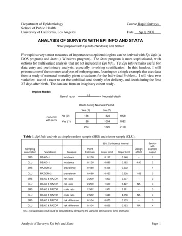
Department of EpidemiologySchool of Public HealthUniversity of California, Los AngelesCourse Rapid SurveysDateSp Q 2008ANALYSIS OF SURVEYS WITH EPI INFO AND STATANote: prepared with Epi Info (Windows) and Stata 8For rapid surveys most measures of importance to epidemiologists can be derived with Epi Info (aDOS program) and Stata (a Windows program). The Stata program is more sophisticated, withoptions for multivariate analysis that are not included in Epi Info. Yet Epi Info remains useful fordata entry and preliminary analysis, especially involving stratification. In this handout, I willpresent some of the common analyses of both programs, focusing on a single example that uses datafrom a study of neonatal mortality given to students for the Individual Problem. I will view twovariables: use of a razor to cut the umbilical cord shortly after delivery, and death during the first27 days after birth. The data are from an imaginary cohort study.Implied Model:Use of razor(-) Neonatal deathDeath during Neonatal PeriodCut cordwith razorYes (1)No (2)No (2)1868221008Yes (1)881004109227418262100Table 1. Epi Info analysis as simple random sample (SRS) and cluster sample (CLU).PointEstimateLower LimitUpper LimitDesigneffectSectionwithexampleoutput95% Confidence D 1incidence0.1300.1170.146--1CLUDEAD 1incidence0.1300.0990.1624.402SRSRAZOR 2prevalence0.4800.4580.502--1CLURAZOR 2prevalence0.4800.4520.5081.632SRSDEAD & RAZORrisk ratio2.2901.8032.907--3CLUDEAD & RAZORrisk ratio2.2901.5303.427NA4SRSDEAD & RAZORodds ratio2.5821.9713.381--3CLUDEAD & RAZORodds ratio2.5821.6404.058NA4SRSDEAD & RAZORrisk difference0.1040.0750.133--3CLUDEAD & RAZORrisk difference0.1040.0550.153NA4NA not applicable (but could be calculated by comparing the variance estimates for SRS and CLU)Analysis of Surveys: Epi Info and StataPage 1
Table 2. Stata analysis as simple random sample (SRS) and cluster sample (CLU).PointEstimateLower LimitUpper LimitDesigneffectSectionwithexampleoutput95% Confidence D 1incidence0.1300.1160.145--5CLUDEAD 1incidence0.1300.0990.1624.3986SRSRAZOR 1prevalence0.4800.4590.501--5CLURAZOR 1prevalence0.4800.4520.5081.6326SRSDEAD & RAZORrisk ratio2.2901.7772.951--7CLUDEAD & RAZORrisk ratio2.2901.5303.4272.6198SRSDEAD & RAZORodds ratio2.5821.9713.381--9CLUDEAD & RAZORodds ratio2.5821.6424.0582.58010SRSDEAD & RAZORrisk difference0.1040.0750.133--11CLUDEAD & RAZORrisk difference0.1040.0550.1532.62412Analyses with Epi Info1. Under Analysis Commands, the Options command for Statistics is set to Advanced. Then underStatistics the Frequencies command is used for DEAD and RAZOR.FREQ DEADFREQ RAZOR2. Under Analysis Commands, the Advanced Statistics option for Complex Sample Frequencies isused for DEAD and RAZOR.Analysis of Surveys: Epi Info and StataPage 2
FREQ DEAD PSUVAR CLUSTERFREQ RAZOR PSUVAR CLUSTER3. Under Analysis Commands, the Statistics option for Tables is used to compare RAZOR(exposure variable) with DEAD (outcome variable). First, however, RAZOR is recoded from1 and 2 to no and yes so that it lines up correctly in the Epi Info table [note: “no” is exposed tothe risk of neonatal mortality from not using a razor to cut the umbilical cord].Analysis of Surveys: Epi Info and StataPage 3
RECODE RAZOR TO RAZOR1 "Yes"2 "No"ENDTABLES RAZOR DEAD4. Under Analysis Commands, the Advanced Statistics option for Complex Sample Tables isused to compare RAZOR (exposure variable) with DEAD (outcome variable). As before,RAZOR is recoded from 1 and 2 to no and yes so that it lines up correctly in the Epi Infotable.Analysis of Surveys: Epi Info and StataPage 4
TABLES RAZOR DEAD PSUVAR CLUSTERAnalyses with Stata5. The variables DEAD and RAZOR in the Epi Info file were recoded from the original valuesof 1 and 2 for DEAD to 1 (dead) and 0 (alive) and for RAZOR to 1 (not used) and 0 (used).The *.mdb file was then saved as a *.rec file (named with 8 letters or less), moved to theDATA subdirectory in Stata, and converted to a *.dct file with the epi2dct.exe program.Thereafter the *.dct file was read into Stata with the infile using command and saved as a*.dta file. Once in Stata, the means of the binomial variables DEAD and RAZOR wereanalyzed as if the data came from a simple random sample.means dead razor6. To analyzed the means correct as a cluster survey, the primary sampling unit (PSU – cluster)needs to be recognized. The recognition is created with the svyset, psu(cluster) command,followed by svymean dead razor to derive the means.Analysis of Surveys: Epi Info and StataPage 5
svymean dead razor7. For the risk ratio, first assume the data were derived from a simple random sample. Tocalculate the risk ratio comparing RAZOR (the exposure variable coded as 1 for not used and0 for used) to DEAD (the outcome variable coded as 1 for dead and 0 for alive), the poissonregression command is used.poisson dead razor, irr8. Next correctly assume the data were derived from a cluster survey. To calculate the riskratio comparing RAZOR to DEAD, the survey version of the poisson regression command isused.svypois dead razor, irr ci deff9. For the odds ratio, first assume the data were derived from a simple random sample. Tocalculate the odds ratio comparing RAZOR (the exposure variable coded as 1 for not usedand 0 for used) to DEAD (the outcome variable coded as 1 for dead and 0 for alive), thelogistic regression command is used.Analysis of Surveys: Epi Info and StataPage 6
logit dead razor, or10. Next correctly assume the data were derived from a cluster survey. To calculate the oddsratio comparing RAZOR to DEAD, the survey version of the logistic regression command isused.svylogit dead razor, or ci deff11. For the risk difference, first assume the data were derived from a simple random sample. Tocalculate the risk difference comparing DEAD (coded as 1 for dead and 0 for alive) amongRAZOR coded as 1 (i.e., not used) versus RAZOR coded as 0 (i.e., used), the binomialregression command is used.binreg dead razor, rd12. Lastly, correctly assume the data were derived from a cluster survey. To calculate the riskdifference comparing DEAD (coded as 1 for dead and 0 for alive) among RAZOR coded as 1(i.e., not used) versus RAZOR coded as 0 (i.e., used), the linear regression command is used.Analysis of Surveys: Epi Info and StataPage 7
svyregress dead razor, ci deffAnalysis of Surveys: Epi Info and StataPage 8
Epi Info analysis as simple random sample (SRS) and cluster sample (CLU). Sampling assumption 95% Confidence Interval Design effect Section with example Variable(s) Measure output Point Estimate Lower Limit Upper Limit SRS DEAD 1 incidence 0.130 0.117 0.146 -- 1 CLU DEAD 1 incidence 0.130 0.099 0.162 4.40 2 SRS RAZOR 2 prevalence 0.480 0.458 0 .