Transcription
FOLDBLEEDBLEEDSignificant data providersPetróleos MexicanosU.S. National Oceanic and Atmospheric AdministrationBLEEDFOLDBLEED
Carte des Anomalies Magnétiques de l’Amérique du NordMagnetic Anomaly Map of North AmericaMapa de la Anomalía Magnética de NorteaméricaProcessing, Compilation, and Geologic Mapping Applications of theNew Digital Magnetic Anomaly Database and Map of North AmericaBy North American Magnetic Anomaly Group (NAMAG)Viki Bankey2Alejandro Cuevas3David Daniels2Carol A. Finn2Israel Hernandez3Patricia Hill2Robert Kucks2Warner Miles1Mark Pilkington1Carter Roberts2Walter Roest1Victoria Rystrom2Sponsored by1Geological Survey of Canada2United States Geological Survey3Consejo de Recursos Minerales de México2002Printed byU.S. Department of the InteriorU.S. Geological SurveySarah Shearer2Stephen Snyder2Ronald Sweeney2Julio Velez3
1introductionIntroductionThis digital Magnetic Anomaly database and map for the NorthAmerican continent is the result of a joint effort by the GeologicalSurvey of Canada (GSC), U.S. Geological Survey (USGS), andConsejo de Recursos Minerales of Mexico (CRM). The database andmap represent a substantial upgrade from the previous compilationof Magnetic Anomaly data for North America, now over a decadeold (Committee for the Magnetic Anomaly Map of North America,1987). This integrated, readily accessible, modern digital databaseof magnetic anomaly data will be a powerful tool for further evaluation of the structure, geologic processes, and tectonic evolution ofthe continent and may also be used to help resolve societal andscientific issues that span national boundaries. The North Americanmagnetic anomaly map derived from the digital database providesa comprehensive magnetic view of continental-scale trends not available in individual data sets, helps link widely separated areas ofoutcrop, and unifies disparate geologic studies. This booklet outlinesthe data processing and compilation procedures used to produce themagnetic anomaly database and map that accompany this booklet.
2IntroductionIntroducciónL’actualisation de la banque de données numériques et dela carte magnétique de l’Amérique du Nord est le résultat desefforts conjoints de la Commission géologique du Canada (CGC),du U.S. Geological Survey (USGS) et de Consejo de RecusosMinerales de México (CRM). Cette banque de données moderne,intégrée et facile d’accès couvre toute l’Amérique du Nord; ellesera un outil puissant pour faire de nouvelles interprétation desstructures, des processus géologiques et de l’évolution tectoniquede continent, en outre, on pourra l’utiliser pour résoudre desproblèmes sociaux et scientifiques couvrant plusieurs pays. Lacarte des anomalies magnétiques de l’Amérique du Nord produiteà partir de données numériques fournit une vue, à l’échellecontinentale, de linéaments non identifiables sur des ensemblesséparés de données, elle aide à regrouper des affleurementsséparés de roches et à unifier diverses études géologiques. Cettebrochures donne un aperçu des techniques de compilation et detraitement utilisés, et des applications géologiques possibles àpartir de cette carte magnétique et des données numériques.La actualización de la base de datos digital y el mapa dela anomalía magnética de Norteamérica es el producto de unesfuerzo conjunto entre el Geological Survey of Canadá (GSC),el U.S. Geological Survey (USGS) y el Consejo de RecursosMinerales de México (CRM). Esta base de datos moderna y defácil acceso que comprende todo Norteamérica constituirá unapoderosa herramienta para nuevas evaluaciones de las estructuras,procesos geológicos y evolución tectónica del continente y puedeser usada para ayudar a resolver aspectos sociales y científicosque se extienden mas allá de las fronteras nacionales. El mapade anomalía magnética de Norteamérica derivado de la base dedatos digital proporciona una visión de lineamientos magnéticos aescala continental que no se puede apreciar en los grupos de datosindividuales, ayudando a agrupar afloramientos de rocas ampliamente separados y a unificar estudios geológicos. Este folletodescribe la compilación y procesamiento utilizado para producirla nueva base de datos digital y el mapa de anomalía magnéticade Norteamérica.
3Magnetic Anomaly DataMagnetic anomaly data provide a means of “seeing through”nonmagnetic rocks and cover such as vegetation, soil, desert sands,glacial till, man-made features, and water to reveal lithologic variations and structural features such as faults, folds, and dikes. Magneticanomalies reflect variations in the distribution and type of magneticminerals—primarily magnetite—in the Earth’s crust. Magnetic rockscan be mapped from the surface to great depths, depending on theirdimensions, shape, and magnetic properties, and on the characterof the local geothermal gradient. In many cases, examination ofmagnetic anomalies provides the most expeditious and cost-effectivemeans to accurately map geologic features in the third dimension(depth) at a range of scales.Publicly available airborne and marine magnetic data have beencollected in North America primarily by the governments of Canada,the U.S., and Mexico. In the early 1980’s, the first magnetic anomalymap was produced for the U.S. (Zietz, 1982). A digitized version ofthis analog map constitutes most of the data for the conterminous U.S.in the North American magnetic anomaly map compilation (Committee for the Magnetic Anomaly Map of North America, 1987),constructed as part of the Geological Society of America’s Decadeof North American Geology (DNAG) program. The Canadian component of the DNAG map was based on a 2-km grid (Dods and others,1987) covering 70 percent of Canada, with the largest data gaps overwestern Canada and the Arctic Islands. No data over Mexico werepublished in the DNAG map. Although this first Magnetic Anomalymap was a pioneering effort when it was first constructed in analogform, data resolution is sometimes poorly represented, and the mapis often inadequate for addressing current socioeconomic problemsrequiring modern digital analysis. Moreover, the analog techniquesused to assemble the data did not properly reconcile the disparateflight specifications of individual surveys, resulting in substantialinconsistencies that became more obvious after the data had been digitized (Committee for the Magnetic Anomaly Map of North America,1987; National Research Council, 1993). As a result of these pastcompilation problems and recent major improvements in data coverage, primarily in Canada and Mexico, an effort to compile a newdigital database covering North America was clearly warranted andwas one of the key recommendations of the U.S. Magnetic AnomalyData Set Task Group (1994), who developed the rationale and operational plan for improving this data resource.
4Canadian DataCanada has conducted a systematic aeromagnetic mapping program since 1947 (fig. 1) (Teskey and others, 1993), often on a costsharing basis between Federal and Provincial governments. Currently,surveys are contracted out by the GSC and are often jointly funded withindustry partners from both the petroleum and mining sectors. Mostsurveys (70 percent of land coverage) were flown at a line spacing of0.8 km (fig. 2) and flight height of 0.3 km above the terrain. Detailedmapping at line spacings as small as 0.2 km and regional surveysover sedimentary basins at line spacings as large as 3 km have alsobeen carried out (fig. 2). Approximately 20 percent of the survey datathat are part of the new Magnetic Anomaly Map of North Americawere digitally acquired; the remaining surveys were digitized from1:50,000-scale magnetic contour maps (for example, fig. 3). Datasources also include ship-borne surveys off the Pacific and Atlanticcoasts, donated gridded data sets from industry, and U.S. Navy airbornesurveys in the Arctic Ocean. Data are maintained in a national aeromagnetic database containing over 12,000,000 km of flight-line data andare available in several formats (see http://gdcinfo.agg.nrcan.gc.ca). Inthe period 1988–1999 after the DNAG compilation, the GSC has flown57 surveys acquiring 2,300,000 line-km of magnetic data. Coverage ofwestern Canada and the Arctic has improved significantly.The leveling and merging of aeromagnetic surveys in Canada toproduce a country-wide compilation were started in the late 1970’s.A second phase was started in the late 1980’s and has continued,resulting in a regional compilation for most of the Canadian landmassand offshore areas (Teskey and others, 1993). As part of the newNorth American map, additional data (mostly over the Arctic Islands)were merged with the existing database to produce the most up-todate coverage of the country.Procedures and software used to compile the 1-km grid of magnetic data for Canada are detailed on the Geophysical Data Centrewebsite (http://gdcinfo.agg.nrcan.gc.ca) and are briefly summarizedhere. For areas with flight-line data coincident with the existing 2-kmnational grid (Dods and others, 1987), the difference between the2-km grid and the gridded flight line was used to determine a firstorder correction (either a constant value or a first-order surface). Forsurveys constituting new coverage, this correction was determinedthrough overlap with surrounding surveys. In both cases, the International Geomagnetic Reference Field (IGRF) for the year and altitudeat which the survey was flown was subtracted from the flight-linedata. To generate seamless, discontinuity-free boundaries between thesurveys, differences between surveys were determined in the overlapregion and apportioned over a border zone at the survey boundaries.Merging surveys flown at a constant elevation above topography withsurveys flown at a constant altitude was achieved by computationallydraping data from the constant-altitude surveys to a surface 305 mabove topography using the method of Cordell (1992). Some areas,such as the Yukon Territory, were acquired during periods of highdiurnal variations in the Earth’s magnetic field, a hazard of surveyingin the auroral zone. To reduce the effects of these secular variationsin the Earth’s magnetic field, the survey grids were decorrugated ormicro-leveled. This involved a directional filter that reduces anomalies in the flight-line direction. Flight-line data and various grid products can be obtained from the Geophysical Data Centre website(http://gdcinfo.agg.nrcan.gc.ca).
5
6Figure 1. Beechcraft Queenair B80 aircraft of the Geological Survey ofCanada equipped with a twin magnetometer system (separation 2 m) formeasuring the vertical gradient of the magnetic field. Photographed in 1973.Courtesy Geological Survey of Canada.
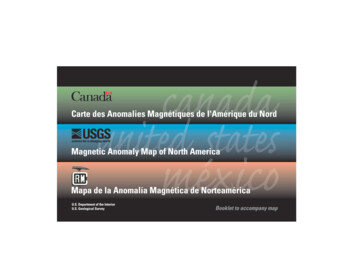
785 80 75 70 65 60 55 50 45 0 14FLIGHT-LINE SPACING40 40 1.0 km or less3.3–7.9 km1.1–2.0 km8.0 km or greater2.1–3.2 kmGridded data 13500 60 120 110 100 90 80 70
8United States DataFigure 3 (above). Example of hand contouring of analog magnetic profiledata. Courtesy Consejo de Recursos Minerales of Mexico.Figure 2 (facing page). Index map showing flight-line spacings of magneticsurveys used in the Canadian part of the North American grid.The USGS pioneered the first airborne magnetic survey in 1945(fig. 4). Subsequently, the USGS has acquired aeromagnetic data (fig.4) for essentially all of the U.S. in a piecemeal fashion. Surveyswere designed for many purposes, so they varied widely in bothsize of coverage and anomaly resolution (determined primarily fromflight height and line spacing) (fig. 5). Data collection methodsspanned changes in acquisition techniques, from analog-based beforethe 1970’s (for example, fig. 6) to current digital systems utilizingGlobal Positioning System (GPS) navigation (for example, fig. 7).After more than 50 years, the USGS’s digital and analog archives ofaeromagnetic data comprise more than 1,000 surveys consisting ofnearly 8,000,000 line-km of data that would cost hundreds of millionsof dollars to re-fly today.For the national compilation that forms part of the North Americandatabase, the USGS has constructed a data set containing the originalaeromagnetic survey data (in digital form) from surveys, maps, andgrids of existing public-domain and, where available, proprietary magnetic data (about 5,800,000 line-km). These data either exist as digitallyprocessed flight-line data (here called digital data) or were derivedfrom analog maps if the flight-line data were not available (calleddigitized data). In the latter case, the analog maps (for example, fig.3) were digitized, generally taking points from intersections of flightlines with magnetic contour lines and their maximum and minimumvalues. Where required, further digitizing was done to augment valuesalong flight lines. Most of the aeromagnetic data were usually correctedduring initial processing for the diurnal variations of the magneticfield, lag, heading, and occasional errors in flight-line elevation. Thesecorrections are often not retained in the original digital data files.
9
10Figure 4. A (pages 9–10). The U.S. Geological Survey (USGS) pioneered the first airborne magnetic survey in 1945 using this Beechcraft Staggerwing 17aircraft. Note the magnetometer “bird” suspended below the aircraft. (Two views of the same aircraft.) B (pages 11–12). This twin-engine Beechcraft ownedby the USGS was used for magnetic surveys throughout the United States in the 1940’s and 1950’s. C (pages 13–14). Two views of a Convair 240 acquired in1963 by the USGS and used for magnetic surveys over the United States until 1971. Note the “tail stinger,” which was retractable and held the magnetometer.D (pages 15–16). These DeHavilland Beavers were acquired in the early 1970’s by the USGS for use in magnetic surveys, but were used for only a few years.U.S. Geological Survey photographs.
11
12
13
14
15
16
17Over the last 16 years, these survey data have been reprocessed,gridded, and merged into regional compilations at U.S. State scales.Many States have been digitally compiled over the last decade(for progress on State compilations, go to http://crustal.usgs.gov/namad/ ). Information on the details of the data processing stepsfor each State and regional compilation that comprise the U.S. Magnetic Anomaly grid can be found in individual reports (see x.html for list). Surveyscovering small areas ( 10 km by 10 km) were generally not includedin the State compilations.Grids were constructed from the original aeromagnetic surveydata with a cell size between one-third and one-fifth of the flight-linespacing of the survey using a bi-directional gridding algorithm. Fordigitized contour line data, the initial grid was constructed using aminimum curvature algorithm with a grid cell size appropriate forthe scale of the digitized map. Usually the Definitive GeomagneticReference Field (DGRF), in conjunction with the International Geomagnetic Reference Field (IGRF) 1990, was applied for the dateof the original survey. However, for some surveys flown before theoriginal IGRF series of main field models were available, GoddardSpace Flight Center (December 1966) or any of several variationsof Polar Orbiting Geophysical Observatory models were used. Theoriginal IGRF1965 model was used often after its availability in 1968.IGRF1975 came out a decade later, followed by IGRF1980. After this,the DGRF suite of models was born out of necessity for creating auniform standard. Whenever possible, these and other original modelswere first added back to the survey data, then the appropriate DGRFwas removed.The survey grids were resampled, as necessary, to final cellsizes of 500 and 1,000 m using a minimum curvature algorithm. Theoriginal grids were upward or downward continued and convertedfrom level to drape (Cordell, 1992), as necessary, to produce a consistent survey specification of 305 m (1,000 ft) above the terrain. Theconverted grids were then adjusted by constant values to minimizedifferences at the boundaries.These intermediate compilations were stitched together to form aquasi-consistent grid of data for the U.S. with a spacing of 1 km usingone of two methods. One method applies a function that “blends” thegrids over the area of overlap so that transition from one to the otheris smooth without changing the grids beyond the overlap regions.Another method defines a “suture” within the overlapping area ofthe two grids along which the mismatch in the grid values must becorrected by adjusting the grids on either side of the path, ensuringthat the transition from one grid to the other remains smooth, nomatter the amplitude and wavelength of the features that the suturepath crosses. In general, suture was the method of choice, becauseit seemed to modify the data mostly in the middle of the overlapzone, and then quickly honor the original data in both grids as onemoved away from the suture. But suture also had the drawback ofoften leaving an artificial anomaly along the suture zone. Wheneverthis was apparent, and not easily corrected, the grid-knit blend optionwas used, generally merging the data admirably, but also modifyingthe data in both grids further from the center of the overlap zone.Figure 5 (facing page). Index map showing flight-line spacings of magneticsurveys used in the U.S. part of the North American grid.
18FLIGHT-LINE SPACING1.0 km or less1.1–2.0 km120 2.1–3.2 km110 4.8–8.0 km70 100 90 45 45 8.0 km or greater80 40 40 70 53 35 ALASKA70 120 66 30 110 62 20 162 19 156 155 58 156 150 144 138 132 HAWAII30 90 100 80
19Mexican DataAeromagnetic surveys in Mexico have been flown by CRM insupport of mineral exploration since 1962 (figs. 6, 7, and 8). Priorto 1992, the surveys were flown along north- and northeast-trendingflight lines spaced 800–1,000 m apart with flight heights of 120,300, and 450 m above the terrain (fig. 9). The data were plottedon 1:50,000-scale contour maps (fig. 3) and then digitized by hand,producing about 360,000 line-km of digital data. The points weredigitized from intersections of flight lines with magnetic contour linesand their maximum and minimum values. Where required, furtherediting was done to the line data. The Definitive Geomagnetic Reference Field (DGRF) was subtracted using the digital elevation modeland the year and altitude of each survey. Grids were constructed fromthe database with a cell size one-fifth that of the flight-line spacing,using a minimum curvature algorithm. A first vertical derivative filterwas applied to the data to highlight poorly merged areas. These areaswere then re-leveled.Since 1994, the CRM has been systematically flying surveys(fig. 10) over the country’s mining exploration areas with Cesiummagnetometers positioned by differential GPS (fig. 7) along northsouth-trending flight lines spaced 1,000 m apart. The flight heightvaries from about 300 to 450 m above the terrain. The digital information is corrected for the diurnal variations of the magnetic field, lag,heading, DGRF/IGRF, and tie-line mis-ties. It was then microleveled.The original data from the modern digital surveys, as well as the olderanalog data, are available (see http://www.coremisgm.gob.mx).
20Figure 6 (facing page). Analog-based magnetic data were collected before the 1970’susing equipment such as this Gulf Mark IIImagnetometer. Courtesy Consejo de Recursos Minerales of MexicoFigure 7 (left). Cockpit of modern BrittenNorman Islander aircraft equipped with thelatest in digital magnetic data acquisitionsystem and Global Positioning (GPS) navigation. Courtesy Consejo de Recursos Minerales of Mexico.
21
22Figure 8 (facing page). The first aircraft used by Consejo de RecursosMinerales of Mexico for magnetic surveys from 1962 to 1974 was this ScottishAviation Twin Pioneer equipped with a Gulf Mark III magnetometer. Seefigure 6 for photograph of a Gulf Mark III magnetometer. Courtesy Consejo deRecursos Minerales of Mexico.
23114 32 108 102 28 28 114 24 108 24 90 FLIGHT HEIGHT120 mFLIGHT-LINE SPACING800 m or less20 20 300 m1 km450 m1 km20 20 90 102 Barometric1 km gridded data16 16 Lighter shades of red, orange, and yellow indicate digitized data96
24Offshore DataFor the national compilation that is part of the North Americandatabase, all of the CRM grids, originally gridded with a cell size onefifth that of the line spacing, were downward or upward continued to305 m above ground level and resampled to a 200-m grid. Each gridwas adjusted by an appropriate constant to minimize differences atsurvey boundaries during the process to merge adjacent surveys.The National Oil Company (PEMEX) provided 19 grids, with1-km cell size, covering southeast Mexico. The surveys were flownwith line spacings ranging from 2 to 6 km and flight heights from 450to 3,350 m above sea level. These data were reprocessed to accountfor the IGRF. Each individual grid was converted from a constant(barometric) altitude to a constant elevation above terrain, then apolynomial of first degree was removed before merging all of theindividual grids. This final grid (gray areas in fig. 9) was merged withthe CRM grid to generate the Mexico magnetic grid.Figure 9 (facing page). Index map showing flight heights and flight-line spacings of magnetic surveys used in the Mexican part of the North American grid.Since the DNAG compilation, the offshore data coverage hassignificantly improved. These improved data have been incorporatedwith the aeromagnetic data for this map. The marine data wereobtained from the National Geophysical Data Center of the NationalOceanic and Atmospheric Administration and span the years 1958through 1997. Only total magnetic field data were used, to whichdiurnal corrections, when available, had already been applied. TheDGRF was then removed, using the date of the original surveys.These data were then heavily edited, removing obvious erroneousstations and surveys. Gridding was performed to a final cell size of1 km using a minimum curvature algorithm and a grid radius of 24km to fill in the many small no-data areas. This final grid was thentrimmed, removing those data areas which overlapped the Canadaand United States offshore grid areas (figs. 2 and 5). A slight overlapprovided a smooth transition when merging with adjacent grids.
25Figure 10. This fleet of Britten-Norman Islander aircraft, which is equipped with the latest data acquisition systems, has been used by Consejo de RecursosMinerales of Mexico since 1994. See figure 7 for cockpit view of one of these aircraft. Courtesy Consejo de Recursos Minerales of Mexico.
26
27The North America Magnetic Anomaly Grid and Map ProductsProducts from the North American project include the individualgrids from Canada, the U.S., Mexico, the Arctic (Macnab and others,1995), and marine data. If necessary, each national 1-km grid wasreprojected to the DNAG projection (spherical transverse mercator,central meridian of 100 W., base latitude of 0 , a scale factor of0.926, and Earth radius of 6,371,204 m) (Snyder, 1987; Committeefor the Magnetic Anomaly Map of North America, 1987) and mergedtogether, using both blending and suturing approaches to form theNorth American merged magnetic grid.Although the North American merged grid represents a significant upgrade to older compilations, the existing patchwork ofsurveys is inherently unable to accurately represent anomalies withlong (greater than about 150 km) wavelengths, particularly in the U.S.and Canada (U.S. Magnetic Anomaly Data Set Task Group, 1994).The lack of information about long-wavelength anomalies is primarilyrelated to datum shifts between merged surveys. These shifts arecaused by data acquisition at widely different times and by differencesin merging procedures. The artifacts produced by the shifts havewavelengths the size of one or more survey areas and the amplitudescan easily exceed 100 nT. Reliable measurement of long-wavelengthanomalies is limited by individual survey sizes, regardless of dataquality (for example, it is difficult to definitively measure anomalywavelengths greater than 100 km when the dimension of the surveyarea is less than 100 km).Because wavelengths greater than about 150 km are unreliable inthe compilation, applying a high-pass wavelength filter would appearto be a viable solution to remove these unreliable wavelengths. However, removing wavelengths less than 500 km from the merged gridcreates artifacts, such as spurious separation of continuous anomalies.Therefore, we removed anomalies with wavelengths greater than 500km from the merged grid to reduce the effects caused by the erroneous long wavelengths and to maintain continuity of anomalies. Thecorrection was accomplished by transforming the merged grid tothe frequency domain, filtering the transformed data with a longwavelength cutoff at 500 km, and subtracting the long-wavelengthdata grid from the merged grid. Other methods (for example, Ravatand others, 2002) using equivalent sources based on long-wavelengthcharacterization with satellite and national high-altitude data can alsohelp correct for the shifts.
28Utility of the CompilationThe 500-km low-pass filtered grid was then color-shaded toform the accompanying map. This filtered grid, the merged grid,the equivalent-source corrected grid (Ravat and others, 2002), andall of the correction grids are available with further processingdetails, along with the individual national grids and digitalsurvey boundary files from GSC (http://gdcinfo.agg.nrcan.gc.ca/toc.html), USGS (http://crustal.usgs.gov/namad), and CRM (http://www.coremisgm.gob.mx/inicio.html) websites. In addition, the ASCIIdata sets for publicly available aeromagnetic surveys for the U.S.are available online or on disk. Digitized data from analog magneticmaps are published by the USGS (1999); digital data from originalmagnetic flight-line data will be published in late 2002 (informationon this data will be available at http://crustal.usgs.gov/namad). Metadata files that provide information about the digital data files for eachsurvey are available at the National Geospatial Data Clearinghouse(http://130.11.52.184/).Understanding the regional geology of the continent can provideinformation useful for a wide variety of applications such as mineraland energy resource assessments, earthquake and landslide hazards,and hydrologic and environmental studies. The size of geologic features that can be resolved with magnetic data depends mostly on theflight-line spacing and elevation above the magnetic sources. Onlybroad, regional magnetic sources such as batholiths ( 3 km wide)can be resolved with coarsely spaced ( 3 km) surveys, while finescale features ( 1 km wide), such as shallow dikes, faults, andfolds, can be resolved with closely spaced ( 500 m), low-altitude( 500 m above terrain) data. Case studies illustrating the utility ofvarious high-resolution surveys ( 800 m line spacing) contained inthe upgraded North American Magnetic Anomaly map are available athttp://crustal.cr.usgs.gov/namad.
29Future UpdatesLow-Altitude DataHigh-Altitude DataThe GSC is currently undertaking aeromagnetic surveys in several parts of Canada. Some of this data acquisition fills in gaps in thenational coverage, while other detailed surveys will provide higherresolution data over areas previously flown. Even though the presentcoverage of Canada appears nearly complete, many areas compriseeither surveys flown with widely spaced flight lines (as much as 6 km)or data donated as grids for which data quality is difficult to assess.The current upgraded database of the U.S. still contains majorproblems due to poor data resolution related to wide flight-line spacing and high flight altitudes (as highlighted by U.S. Magnetic Anomaly Data Set Task Group, 1994). Many existing aeromagnetic surveysin the U.S. are not sufficiently detailed to resolve important geologicfeatures or to merge with higher resolution data from Canada andMexico. Data collected over a large part of the U.S. do not adequatelydefine three-dimensional sources shallower than several kilometersprimarily because of large distances between flight lines. Approximately 90,000 line-km of new data are being collected annually by theUSGS. Continued collection of new low-altitude data will be requiredto produce a more consistent U.S. Magnetic Anomaly map.For Mexico, CRM will continue flying magnetic surveys to complete the national magnetic database, and they will fly higher resolution surveys for mining resource exploration as well as hazard andenvironmental assessments.Although corrections for long-wavelength inaccuracy in themerged magnetic compilation have been made (as described previously), our understanding of the sources of error, particularly in the150–500 km range, is incomplete. In order to measure anomalies inthis wavelength range, consistent magnetic anomaly data must be collected at a high altitude (between 15 and 22 km, with equivalent linespacing) over North America (National Research Council, 1993; U.S.Magnetic Anomaly Data Task Group, 1994). A high-altitude aeromagnetic data set over North America and adjacent offshore regionswould serve two important purposes: one, it would allow the studyof long-wavelength magnetic anomalies, which provide insights inthe tectonic assemblages and regional physical properties of the crustand upper mantle; two, it would provide a consistent, continentalwide datum that can be used to eliminate the datum shifts and longwavelength errors in the merged grid. Such an accurate continentwide datum will improve the continuity of magnetic signatures and,therefore, the validity of the magnetic interpretation that is vital toregional geological mapping.
30AcknowledgmentsThere are many geologic and geomagnetic applications of ahigh-altitude aeromagnetic survey, including but not limited to: Increased understanding of the global geomagnetic field A better reference f
data. To generate seamless, discontinuity-free boundaries between the surveys, differences between surveys were determined in the overlap region and apportioned over a border zone at the survey boundaries. Merging surveys fl own at a constant elevation above topography with surveys fl own at a constant altitude was achieved by computationally