Transcription
www.elsevier.com/locate/ynimgNeuroImage 28 (2005) 1043 – 1055Neuronal spatiotemporal pattern discrimination: The dynamicalevolution of seizuresSteven J. Schiff,a,* Tim Sauer,b Rohit Kumar,c and Steven L. Weinstein daKrasnow Institute, Program in Neuroscience and Department of Psychology, George Mason University, MSN 2A1,Fairfax, VA 22030, USAbDepartment of Mathematics, George Mason University, Fairfax, VA 22030, USAcThomas Jefferson High School for Science and Technology, Fairfax, VA 22312, USAdDepartment of Neurology, Children’s National Medical Center and the George Washington University,Washington DC 20010, USAReceived 26 April 2005; revised 12 June 2005; accepted 23 June 2005Available online 28 September 2005We developed a modern numerical approach to the multivariate lineardiscrimination of Fisher from 1936 based upon singular valuedecomposition that is sufficiently stable to permit widespread application to spatiotemporal neuronal patterns. We demonstrate thisapproach on an old problem in neuroscience—whether seizures havedistinct dynamical states as they evolve with time. A practical resultwas the first demonstration that human seizures have distinct initiationand termination dynamics, an important characterization as we seek tobetter understand how seizures start and stop. Our approach isbroadly applicable to a wide variety of neuronal data, from multichannel EEG or MEG, to sequentially acquired optical imaging data orfMRI.D 2005 Elsevier Inc. All rights reserved.Keywords: Epilepsy; Discrimination; Correlation; Synchrony; Dynamics;MultivariateIntroductionMultivariate canonical discrimination was invented by Fisherin 1936 in order to quantify the static taxonomic classificationof plant species (Fisher, 1936). The method seeks to discriminate between species based on weighting different measurements (such as petal length and width) such that the aggregatedata from different species are maximally separated. Modernimplementations of this technique (Flury, 1997) can be numerically unstable when applied to dynamical measures of EEGdata, when common measures of signal frequency or correlationmay at times have very small absolute numerical values further* Corresponding author. Fax: 1 703 993 4440.E-mail address: sschiff@gmu.edu (S.J. Schiff).Available online on ScienceDirect (www.sciencedirect.com).1053-8119/ - see front matter D 2005 Elsevier Inc. All rights unded by noise and measurement error. We invent a novelapproach to the numerical solution of multivariate discrimination, which is consistent with Fisher’s original results, yetpermits an application to the analysis of neuronal electricalactivity. Our approach can be used in many other settings(EEG, MEG, Optical Imaging, fMRI).Although we frequently define seizures as monolithicallydistinct dynamical entities – ictal as opposed to interictal – ithas long been clear that the characteristics of seizures canchange distinctively during an event. Many seizures behaviorallychange from focal to generalized activity, or from tonic toclonic muscle contractions, and there are characteristic EEGchanges that accompany such transitions. Early work by Kandeland Spencer (1961) revealed at least 3 stages of hippocampalseizures in fornix deafferented cats. Studying EEG, extracellularlocal field potentials, and single intracellular recordings fromuntyped cells from cat cortex following topical penicillinapplication, Matsumoto and Marsan (1964) suggested qualitativesegmentation of seizures into Fonset, development course andend . Ayala et al. (1970) recorded from similar seizures anddemonstrated (see their Fig. 1) an onset phase of seizuresdistinct from a middle tonic and terminal clonic phase. Previouswork quantifying the segmentation of seizures focused on thesymbolic similarities (or dissimilarities) between seizures (Wendling et al., 1996, 1999; Wu and Gotman, 1998), yet theirfindings illustrated that EEG signals, from single channels and inaggregate, changed during the course of a seizure. Today, we havestill never defined dynamically a seizure Fonset stage, and such acharacterization is essential if we are to distinguish a pre-ictal statefrom the start of a seizure with better accuracy (Litt et al., 2001).Similarly, identifying a distinct terminal phase of a seizure wouldbe useful in understanding why seizures stop, and how to hastensuch termination.We here apply to our knowledge the first canonical discrimination analysis to search for dynamically distinct stages of
1044S.J. Schiff et al. / NeuroImage 28 (2005) 1043 – 1055MethodsHuman seizuresFig. 1. Schematic of EEG data analysis. Simulated EEG data voltages areshown above for 3 channels with 4 time points each. Following Hilberttransformation and assignment of a phase angle h i for each data point,shown as blue vectors, the order parameters of average amplitude, r(t i )and phase angle h(t i ) are determined at each time point t i . In addition,the differences between average amplitude Dr(t i ) and angle Dh(t i ) withina data window (200 points for each second of data) are used to calculatethe variance of the Dr(t i ) and Dh(t i ) that create a measure of phasedispersion. As a multichannel system synchronizes, the averageamplitude r(t i ) within a window will increase towards unity, while itsamplitude differences Dr(t i ) go to zero. Similarly, synchronization amongchannels will make average angle differences Dh(t i ) constant. Thus, thevariance of both the amplitude differences Dr(t i ) and average angledifferences Dh(t i ) will decrease towards zero in the synchronous state. Atthe bottom of the figure is shown a schematic of our scheme forsurrogate data construction for 2 channels of data within a data window(200 points, only 4 shown). For each channel with amplitude data, thetime series is cut at a random location within each data window, and the2 segments created are swapped in location. This cutting and swapping isperformed at a different random location for each channel, and theresultant data set subjected to the same correlation analysis as theoriginal data. The randomization and swapping is repeated, and thus anensemble of results obtained for which local correlations are largelydestroyed. For phase data as shown above, the Hilbert transformationwas performed on the entire data set. For phase data, the randomizationsare performed for phase angle time series within each data window,choosing random times to cut each 200 point time series of phases, andswapping the 2 segments. Again, these surrogate phase ensembles areused to generate new order parameters of average amplitude, r(t i ) andphase angle h(t i ) at each time point, as well as their differences Dr(t i )and Dh(t i ), which are used for comparison with the original data set.Note that these block shufflings used to destroy short term correlations inamplitude and phase data are distinct from the random permutations usedto re-label the multivariate points in Figs. 4F and 5F.epileptic seizures in humans. Applying these techniques to humanseizures recorded both from the scalp and intracranially, we find inalmost all cases the identification of unique initiation andtermination stage dynamics, distinct from the persistent middlephase of seizures.All human research was carried out on archived datastripped of patient identifiers. This work was approved asCategory 4 Exempt research by the Institutional Review Boardsof both the Children’s National Medical Center and GeorgeMason University.Seizure start and stop times were chosen using customaryclinical EEG inspection by a Board Certified Neurologist (SLW)and Neurosurgeon (SJS). To fully contain the seizure, the nearestinteger second before the seizure onset, and the nearest integer afterseizure offset, were selected. We as others (Wu and Gotman, 1998)were extremely reluctant to pre-select which electrodes should beemployed for analysis. Our only criteria for exclusion were thepresence of significant artifact in the recording channel. For scalpdata, 23 channels were used according to the standard 10 – 20system. For intracranial recordings, the 4 subjects had 28, 63, 63,and 64 usable channels, respectively.All data were recorded following analog high pass filteringbetween 0.1 and 0.3 Hz, and low pass filtering at 100 Hz, prior todigitization at 200 Hz. Before signal processing, data were passedthrough a 9th order low pass Butterworth filter with a cutofffrequency of 55 Hz in order to prevent 60 Hz power linecontamination from affecting our correlation measures. The meanvoltage offset of each channel was similarly removed prior toanalysis.Dynamical measuresSix dynamical measures were calculated within each nonoverlapping 1 s window of data: total power, total correlation atboth zero and arbitrary time lag, phase amplitude coherence, andphase angle and amplitude dispersion. The choice of these sixFfeatures is rather arbitrary, but our goals were to reflect measuresof synchronization from several semi-independent approaches, andin addition the signal power, which is intimately related to changesin epileptic EEG.Total power was calculated by summing the squared value ofeach voltage value.Two measures reflecting total correlation were calculated. Eachelectrodes’ time series, x i (t), where i indicates channel number,was first-order detrended within each T 1 s window, and then thenormalized crosscorrelation function, c i,j (t), was calculated with upto 1/2 s of lagT 2Xxi ðt Þxj ðt þ sÞt ¼ T 2ci;j ðsÞ ¼0@t ¼T 2X11 2 0ðxi ðtÞÞt ¼ T 22A@t ¼T 2X 211 2xj ðt Þ At ¼ T 2This was performed for all unique channel pairs (i,j), and eitherthe values at zero lag (s 0),S0 ¼nXjci; j ðs ¼ 0Þji;j ¼ 1imj
S.J. Schiff et al. / NeuroImage 28 (2005) 1043 – 1055or the values larger than twice the estimator of standard deviation(Bartlett, 1946; Box and Jenkins, 1976), r ij2(s),r2ij ðsÞSs ¼¼jT 2Xci; i ðsÞcj; j ðsÞs ¼ T 2nXðT þ 1 sÞj;T 2 X Ci; j ðsÞ hð Ci; j ðsÞ 2rij ðsÞÞi; j ¼ 1 s ¼ T 2imjwere summed to yield values S 0 or S s , respectively (h is theHeaviside function). Such measures S reflect the total amount ofcorrelation between all channel pairs within the window. Examplesof such correlation values are seen in Fig. 3C, where the correlationvalue at zero lag is the value in the center of the plots, and thevalues of correlation exceeding twice the standard deviation of theconfidence limit are the values exceeding the red error bars atarbitrary lags. Such arbitrary lags will turn out to be crucial toconsider when propagation delays are present in a system.Phase was calculated in broad-band from Hilbert transformationof each full time series from each electrode (at this stage withoutregard to the smaller 1 s windows).The Hilbert transformisn t eoþVdefined as hðt Þ ¼ p1 lime Y 0 X V tx ðsÞs ds þ Xt þ e tx ðsÞs dt ; wherex(t) is the original signal (Bendat and Piersol, 1986). The Gaboriu(t),analytic signal Z(t) is defined as Z(t) x(t) ih(t) a(t)eand the phase of the signal was obtained as uðtÞ ¼ tan 1 hxððttÞÞ (usinga four-quadrant inverse tangent). A schematic of such an analysis for3 channels of data isPshown in Fig. 1. For each time Pt i in the data, thesum of the cosine, nj ¼ 1 cos uj ðti Þ , and sine, nj ¼ 1 sin uj ðti Þ ,of the phases over all n electrodes was taken, and the average phaseamplitude r(t i ) and average angle h(t i ) were calculated ��!2!2ffiu nnX X 1ur ðt i Þ ¼ tcos uj ðti Þþsin uj ðti Þnj¼1j¼1"hðti Þ ¼ tan 1nX cos uj ðti Þ!þij¼1nX sin uj ðti Þ!#j¼1as illustrated in Fig. 1. The variable r(t i ) is also known as mean phasecoherence (Mormann et al., 2000), and is equivalent to (1 minus the)circular variance (Fisher, 1993). The sequential average angleh(t i )was unwrapped by adding 2p whenever mod[h(t i )] 0.The averageP200 phase amplitude within each 1 s window k,1rk ¼ 200i ¼ 1 ri , was calculated in aggregate from all electrodes.The differences of the average r and h, Dr i (r(t i 1 )) r(t i )) andDh i h(t i 1 ) h(t i ), were calculated within each 1 s window (199differences from 200 points). The phase amplitude and angledispersions are the variance of the differences, var[Dr] and var[Dh],within each window. Changes in phase amplitude dispersion havebeen noted to appear to change during peri-ictal recordings(Mormann et al., 2000). As signals become more coherent in phase,both phase amplitude and angle dispersion should decrease.Discrimination numerical analysisDiscrimination was performed on the sequence of the abovemeasurements, assembled into a matrix Y where the rows are in units1045of time (1 s intervals) and the columns represent the 6 multivariatemeasurements of power, total correlation at zero lag, total correlationat arbitrary lag, phase amplitude average, and phase amplitude andangle dispersion averaged over each second. These values give usdifferent measures of the interaction between channels, reflectinglinear, non-linear, and time lagged interactions due to propagationdelays. Since with the approach that follows, adding additionalmeasures should improve rather than impair our ability to discriminate, we have not sought to extract which measures contribute mostsignificantly to the discrimination strength. Instead, followingdiscrimination, we have examined which measures best characterized the difference between the different stages of the seizures.Since we do not know the best way of partitioning each seizure intoa beginning, middle, and end, we examined all possible combinationsby letting the beginning period range from the first 2 s of the seizure upto the first half of the entire seizure duration, while letting thetermination period range from the entire second half of the seizure tothe final 2 s. Two seconds was imposed as the minimum duration of apartition, and was the minimum discretization for adjusting partitions.Such an extensive Fbrute force sweep of partitions would permit us tofind the optimal partitioning—the one which most separated theseizure dynamically into beginning, middle, and end.For each partitioning, we separated the data matrix Y intocorresponding upper, middle, and lower matrices Y1, Y2, and Y3.The multivariatemeans of these matrices were computed asPNi ȳ ¼ 1ji ¼ 1 yji , where yji are i rows (seconds) from the matrixNj1,2,3. Thecovariance matrices areYj for groups j corresponding PN T8i ¼ N1j i ¼j 1 yji ȳjyji ȳj where T indicates transpose,and the fullPcovariance matrix for the entire data set isN T 8total ¼ NN 12i ¼ 1 ðyi ȳÞ ðyi ȳÞ. Pooled covariance withingroups, 8within was calculated as8within ¼1½ðN1 1Þ81 þ ðN2 1Þ82 þ ðN3 1ÞW3 N1 þ N2 þ N3and the between group variance is thus8between ¼ 8total 8withinFisher (1936) recognized that for any linear combination z Yb, where b is a column vector of coefficients, that the variancevar½z ¼ bT 8total b ¼ bT 8within b þ bT 8between band that separate groups j implies that 8total 8within.Our goal is to find the discrimination function Z(c) that bestemphasizes the between with respect to the within covariances, orin other words to maximize the ratiobT 8total bbT 8between b¼1þ T¼1þaTb 8within bb 8within bover all vectors of coefficients b. Then Z(c) Yb will be theoptimal discriminator, and the maximum a will quantify the excessbetween covariance.Fisher’s insight (Flury, 1997) was that this maximization can beTachieved with a simultaneous spectral decomposition of bbT88betweenbbwithin b 8between bbT HLHT bbT Lb T¼¼amax Tb 8within bb HHT bbT bTMaximizing a leads to k 1,. . .,m orthogonal linearcombinations zk Yc k , where c k are the columns of (HT) 1. is a diagonal matrix, whose values k 1 . . . k m 0 k m 1 . . . k p , where p are the number of variables, in our case 6. Thus,
1046S.J. Schiff et al. / NeuroImage 28 (2005) 1043 – 1055there are m canonical discrimination functions, zk , which arelinear combinations Yc k corresponding to the non-zero eigenvalues k 1,. . .,m .In computing this spectral decomposition, we have found thatinstabilities arise from eigenvalue calculations involving plug inestimates of 8within and 8between using dynamical measures ofEEG. This is a general problem for the application of Fisher’smethod to any multivariate data, and is an impediment to theapplication of this technique to neuronal data such as ours.We will focus on a singular value decomposition (SVD) basedapproach to finding the optimal discrimination functions. SVD is afavorable strategy for efficient matrix computations due to itsfavorable error handling properties. For example, least squarescalculations are often solved by the normal equations in theory, butan approach using the SVD is the preferred choice if the calculationis data intensive, and especially if noisy or uncertain data areinvolved. In essence, the SVD determines a convenient orthogonalchange of basis with which to apply matrix computations. Thecondition number (ratio of largest to smallest singular values) ofsuch matrices determines the sensitivity of such solutions to errorsand noise in the data. The favorable rotation of coordinates andorthogonality of SVD causes inadvertent large projections of smallerrors to be avoided, and helps preserve good ‘‘conditioning’’ ofmultilinear problems. In addition to providing additional stability ofsolutions compared with alternative approaches to discriminantsolutions (Flury, 1997), our use of SVD will have the benefit of atransparent geometry with which to interpret the analysis.The right change of coordinates simplifies the discriminationproblem considerably. Let 8within USUT be the singular valuedecomposition (SVD) of 8within, where S is diagonal, and Uappears twice because covariance matrices are symmetrical. Definea new variable v US1/2UTb, or equivalently b US 1/2UTv. Interms of v,a¼vT US 1 2 UT 8between US 1 2 UT vvT US 1 2 UT 8within US 1 2 UT v¼vT US 1 2 UT 8between US 1 2 UT vvT vThis is a much better coordinate system in which to do themaximization. Since the length of v scales out of the ratio, it isequivalent to maximize over unit vectors v. We know that, ingeneral, the maximum of vTAv for a symmetric matrix A is reachedfor v v1, the first singular vector of A. Furthermore, the maximumsubject to being orthogonal to v1 is v2, the second singular vector ofA, etc. So the maximization is solved by taking the SVDUS 1 2 UT 8between US 1 2 UT ¼ VAVTand the maximum a is v1TVAVTv1 k 1, the largest singular valuefrom A. Converting back to b-coordinates, the optimal b, called thefirst canonical variate, isb1 ¼ US 1 2 UT v1which is the first column of US 1/2UTV. The second column b2 ofUS 1/2UTV is the second canonical variate, and so on. The mcanonical variates b1,. . ., bm , are the m columns of US 1/2UTV.They provide the coefficients of m canonical discriminationfunctions Zi (c) YbTi .Clearly the choice b US 1/2UTv was a good one, but what isthe intuition behind it? The geometry is shown in Fig. 2A. TheFig. 2. Geometry of Fisher canonical discrimination with new approach tonumerical analysis. In panel A, we show schematically the cloud of datapoints from which the within group covariance is derived, 8within. Thesedata are transformed with transformation S to the unit circle in coordinatesU. Similarly, the cloud of mean points from which the covariance 8betweenis derived is transformed into the U coordinate system. An inversetransformation, S 1 is applied to the mean points, so that, for instance,compression (expansion) of within group values along a certain axis is nowapplied as expansion (compression) to separate (bring closer) the means.The mean values are now brought out of the U coordinate system throughUT, and the major and minor axes of the ellipse characterized by k 1 and k 2.We see in panel B how this applies to 2 data sets with 2 means. Each dataset (one red, the other blue) is transformed so that their within groupcovariances, 8within, are unity. Their means (red and blue dots below) arebrought into the U coordinate system, inverse transformed with S 1, andbrought back to their original coordinates. The 3 general cases are shown onthe right side. If the unit covariances and means overlap, then k 1,2 are nearzero, indicating that the means, and hence the groups, are not discriminable.The second case shows where the means are separated by a largest k 1 whichapproaches unity. This case is barely discriminable. Finally, in the lowercase, we see that the means are separated by a largest k 1 which is greaterthan unity. In this latter case, after adjusting the within group covariances tounity, the means remain separable by a large enough distance so that theyare likely to have been selected from groups with different means. This isthe fundamental feature of discriminable groups.
S.J. Schiff et al. / NeuroImage 28 (2005) 1043 – 1055transformation simply scales linearly along the principal axes ofthe within covariance ellipsoid, so as to make the within ellipsoidthe unit sphere. The magnitude of the principal axes of the resultingbetween ellipsoid are the optimal k i .To see this, note that the coordinate change consists of threetransformations. First, use UT to change to the coordinate systemwhere the covariance matrix 8within is a diagonal matrix (where thecorresponding 8between covariance ellipsoid is aligned with thecoordinate pffiffiffiffi 2 axes). Second, shrink the ith coordinate axis by a factorofsi ¼ si . Third, change back to the original coordinatesystem. After these three transformations, the 8within covarianceellipsoid was squeezed to the unit ball, normalizing the withincovariance to better evaluate the size of the 8between covarianceellipsoid. The magnitude of the principal axes of the resulting8between covariance ellipsoid are now the k i , and the semi-majoraxes are in the direction of the bi .Fig. 2B illustrates the 3 general cases from this geometricaltransformation. All within group covariances are transformed intounit spheres. The means of each group are stretched or shrunk byan amount that is the inverse of the transform required to create theunit spheres. On the right hand side, the first case is that theeigenvalues k i approach zero. There is no discrimination possiblebecause the means and covariances of the groups overlap nearlycompletely. The second case is where the eigenvalue k 1 approaches1. Here, the unit spheres are just touching, which is the thresholdfor discriminating 2 groups. In the final case, k 1 1, and the meansof the two groups are separated by more than the within groupcovariances, implying that these data are discriminable into twoseparate groups.Testing discrimination qualityFor each multivariate data vector Y (sample of power, averagephase amplitude, 2 correlation measures, and 2 phase dispersions),the transformed vectors z have means u and normal p-variatedistributions f(z). Prior probabilities p j are determined from thefraction of total samples within group j, p j N j / N. The posteriorprobability p jz is the probability that for a given value of z, that thedata came from group j of n groupspj f j ðzÞ; k ¼ 1;N ; npjz ¼ Xnpk f k ðzÞk ¼ 1A suitable approximation to p j f j (z) is given by exp[ q(z)] whereqðzÞ ¼ uTj z 12 uTj uj þ lnpj (Flury, 1997). The highest posteriorprobability among all possible groups is the predicted groupmembership used in our calculations.A robust method of testing the quality of classification is toleave one multivariate data point out of the calculation of thediscriminant function, and then test for predicted group classification given its posterior probability.A normal theory method to test for the significance ofdiscrimination is to examine the magnitude of the eigenvalues of above. We make use of Wilks’ statistic,W. After calculating thePlog likelihood ratio as LLRS ¼ N mi ¼ 1 lnð1 þ ki Þ, where k i arethe diagonal entries of , W ¼ exp N1 LLRS . A poor discrimination yields small eigenvalues k i , and W approaches 1. Gooddiscrimination yields large eigenvalues, and W becomes small.Since W is chi-squared distributed, we can calculate confidencelimits that the discrimination is significant (Flury, 1997).1047We have compared our new numerical approach with morestandard numerical analysis (Flury, 1997) for the original Fisherdata set of morphometric measurements from 3 different iris flowerspecies. The canonical discrimination functions are, up to anarbitrary sign, identical, and the W calculated by both methods isidentical (and highly significant).Since we derive W from assumptions of normal distribution ofdata variables with equal covariances, which our real data willdeviate from, an alternative means of testing the quality ofdiscrimination is to randomly permute the labeling of eachmultivariate data point (to beginning, middle, or end of seizuregroups), and re-test the goodness of fit. Although there aretheoretically N!/N 1 N 2 N 3 possible combinations for each of thethree groups (where N is the total number of measurements, and N iare the number within each partition), we will limit ourpermutations to 1000.In summary, we will present three different measures of thesubstantiality of discrimination: leave one out error rate, W and itsnormal theory confidence limits, and a bootstrapped confidencelimit that is robust against deviations from normality in the datastructure.A full copy of working source code (written in Matlab) alongwith a data sample (Scalp subject B, from Fig. 4) is archived asSupplementary data).Models of coupled systemsIn order to help interpret our findings, we will also buildsequentially more complex linear autoregressive (AR) models ofcoupled systems. These systems and resulting analysis areillustrated in Fig. 3. We started with a 4 channel AR system, andby brute force progressively increased the complexity in order tocreate the simplest linear systems capable of replicating ourfindings. The simplest AR model isx1 ðtÞ ¼ ax1 ðt 1Þ þ n1 ðt Þx2 ðtÞ ¼ ax2 ðt 1Þ þ n2 ðt Þx3 ðtÞ ¼ ax3 ðt 1Þ þ n3 ðt Þx4 ðtÞ ¼ ax4 ðt 1Þ þ n4 ðt Þwhere for 4 channels of simulated data, x(t)1. . . x(t)4, each valueat time t is coupled to the previous value within the channel attime t 1, with the addition of an independent Gaussiandistributed random value n(t). The model is seeded with randominitial conditions. This model generates a data set withoutcoupling between the 4 channels.Our next AR model of interest will bex1 ðtÞ ¼ ax1 ðt 1Þ þ bx2 ðt 1Þ þ n1 ðt Þx2 ðtÞ ¼ ax2 ðt 1Þ þ n2 ðt Þx3 ðtÞ ¼ ax3 ðt 1Þ þ bx4 ðt 1Þ þ n3 ðt Þx4 ðtÞ ¼ ax4 ðt 1Þ þ n4 ðt Þwhere the first channel is coupled to the second, and the thirdchannel is coupled to the fourth, but there is no coupling betweenchannels 1 and 2 with channels 3 and 4.
1048S.J. Schiff et al. / NeuroImage 28 (2005) 1043 – 1055The final AR model is more complexx1 ðt Þ ¼ ax1 ðt 2Þ þ bx2 ðt 2Þ þ cx2 ðt 4Þ þ dx2 ðt 6Þ þ n1 ðt Þx2 ðt Þ ¼ ax2 ðt 2Þ þ n2 ðt Þx3 ðt Þ ¼ ax3 ðt 2Þ þ bx4 ðt 2Þ þ cx4 ðt 4Þ þ dx4 ðt 6Þ þ n3 ðt Þx4 ðt Þ ¼ ax4 ðt 2Þ þ n4 ðt ÞHere, there are significant propagation delays in the couplingboth within each channel, and between channels. Again, onlychannels 1 and 2 and channels 3 and 4 are coupled to eachother.ResultsOur discrimination analysis (see Methods) functions geometrically by renormalizing the covariances of each group’s withingroup covariance, and disentangling the overlap between groupmixtures so that the separation of group means is maximal (Fig. 2).Twenty-four seizures (12 scalp, 12 intracranial) were studied forthe presence of significantly discriminable beginnings, middles,and ends.Twelve scalp seizures were selected for detailed analysis, from79 consecutive scalp seizure records (excluding those with onlyabsence or myoclonic seizures), because they were sufficiently freeof artifact (determined by two investigators) to permit detaileddynamical study. The remaining scalp recordings utilized standard10 – 20 electrode placement obtained from 5 children (labeled
S.J. Schiff et al. / NeuroImage 28 (2005) 1043 – 1055subjects A through E) 2.3 to 12 years of age. One child hadcryptogenic generalized seizures not being treated at the time of therecording and the others were receiving 2 – 3 anticonvulsants. Thesymptomatic seizures were a consequence of bi-occipital gliosis,cerebellar atrophy with history of prior hemiparesis, bi-parietalencephalomalacia and ventriculomegaly, and cortical laminardisorganization with dysgenic hippocampus. Each child had 1 – 5partial seizures with or without secondary generalization analyzed.The montage and an example from one subject (scalp subject B)are shown in Figs. 4A and B.Twelve intracranial seizure records from 4 patients (labeled Athrough D) with disparate seizure types and etiologies werewithout significant electrical artifact (from 16 consecutive records)and were selected for further study. Subject A had a dysplasticposterior temporo-parietal cortex, subject B had frontal gliosis,subject C had a small cortical low grade astrocytoma with highlyfocal seizures confined to a several square centimeter region nearthe tumor, and subject D had both a dysplastic occipital lobe andmesial temporal sclerosis (Fig. 5A). An example of a seizure fromsubject D is shown in Fig. 5B. Of 16 consecutive intracranialseizures for these patients, 12 were selected as free from artifactafter no more than 1 bad channel was eliminated from analysis. Inall, 3 seizures were selected for each of the 4 intracranial subjects.Examples of the dynamical data calculations without regard todiscrimination are shown in Figs. 4E and 5E. We examined allpossible partitions of such data to divide the seizure into beginning,middle, and terminal segments. This is done by letting thebeginning period vary from 2 s to up to half of the seizure inlength, and similarly letting the terminal period vary from the last
of both the Children's National Medical Center and George Mason University. Seizure start and stop times were chosen using customary clinical EEG inspection by a Board Certified Neurologist (SLW) and Neurosurgeon (SJS). To fully contain the seizure, the nearest integer second before the seizure onset, and the nearest integer after