Transcription
The Decision to Move House andAggregate Housing-Market Dynamics L. Rachel Ngai†Kevin D. Sheedy‡London School of EconomicsLondon School of EconomicsMay 2019AbstractUsing data on house sales and inventories, this paper shows that housing transactions aredriven mainly by listings and less so by transaction speed, thus the decision to move house iskey to understanding the housing market. The paper builds a model where moving house isessentially an investment in match quality, implying that moving depends on macroeconomicdevelopments and housing-market conditions. The number of transactions has implicationsfor welfare because each transaction reduces mismatch for homeowners. The quantitativeimportance of the decision to move house is shown in understanding the U.S. housing-marketboom during 1995–2003.JEL classifications: D83; E22; R31.Keywords: housing market; search and matching; endogenous moving; match qualityinvestment; mismatch. Weare grateful to the editor and four anonymous referees, and Elliot Anenberg, Johannes Boehm, PaulCarrillo, Adam Guren, Allen Head, Yannis Ioannides, Boyan Jovanovic, Steven Laufer, Kurt Mitman, ChrisPissarides, Morten Ravn, Richard Rogerson, Rob Shimer, and Ben Williams for helpful comments. Wethank Lucy Canham, Thomas Doyle, and Lu Han for providing data. We also thank seminar participants atAtlanta Fed, Bank of Canada, Bank of England, U. Bern, Boston U. Carlos III, U., CREI, EUI, GWU-FRBReal Estate Seminar, U. Helsinki, U. Hong Kong, IIES, U. Louvain, U. Mannheim, Norwegian BusinessSchool, São Paulo School of Economics, Southwest U. of Finance and Economics, Stockholm School ofEconomics, Sveriges Riksbank, Trinity College Dublin, UCL, the Anglo-French-Italian macroeconomicsworkshop, Conference on Research on Economic Theory and Econometrics, ESSIM, HULM — St. Louis,Midwest Macro Meeting, NBER Summer Institute, Search and Matching Network annual conference, SED,and U. Toronto for their comments. Rachel Ngai acknowledges support from the British Academy MidCareer Fellowship. This paper was previously circulated under the title “Moving House”.† LSE, CEPR, and CfM. Email: L.Ngai@lse.ac.uk‡ LSE and CfM. Email: K.D.Sheedy@lse.ac.uk
1IntroductionTransactions in the housing market generate gains from trade by reducing mismatch between housesand their owners’ preferences. There are sizeable fluctuations in the aggregate number of transactions of a comparable magnitude to fluctuations in house prices. The objective of this paper is tounderstand what drives these changes in aggregate housing-market transactions.Housing transactions can be decomposed as the product of how quickly houses are sold and howmany houses are on the market for sale. The stock of houses for sale depends not only on past salesrates, but also on how frequently houses come on to the market. This frequency is affected both bychanges in the total housing stock and homeowners’ decisions to put existing houses up for sale.The first contribution of this paper is to present evidence establishing that the main driverof transactions is changes in how frequently houses come on to the market. Furthermore, U.S.data show that the dominant factor in explaining the number of houses coming on to the marketis homeowners’ decisions to move house, rather than changes in the total housing stock. Thusunderstanding the decision to move house is crucial for explaining changes in transactions. Thesecond contribution of the paper is to build a model based on the idea that moving house constitutesan investment in the quality of the match between a homeowner and a particular house. Whencalibrated to the U.S. economy, the model of moving house is able to generate a substantial increasein housing-market transactions as seen during the housing-market boom of 1995–2003 in responseto changes in macroeconomic conditions.The claim that the moving rate of homeowners is of much greater importance for transactionsthan the selling rate of houses on the market can be understood with some minimal empiricaldiscipline combined with a basic stock-flow accounting identity. Compared to the average timehomeowners spend in a house (more than a decade), the average time taken to sell a house is veryshort (a few months). This means the average sales rate is around thirty times larger than theaverage moving rate, and the stock of houses for sale is about thirty times smaller than the stock ofall occupied houses. An increase in the sales rate with no change in the moving rate would rapidlydeplete the stock of houses for sale leaving little overall impact on transactions, except during ashort transitional period. On the other hand, an increase in the moving rate adds to the stock ofhouses for sale, which increases transactions even with no change in the sales rate.Measures of the moving and sales rates are constructed for the period 1989–2013 using data onsales and inventories of existing single-family homes and the total housing stock. A counterfactualexercise derives the number of transactions that would have occurred if only one of the sales rate,moving rate, or housing stock had varied as in the data, while the other two were held constant attheir average values. This exercise confirms the claim that the moving rate is the dominant factorin explaining changes in transactions. It also shows that changes in the housing stock account forless than a third of the rise in transactions. Since variation in the owner-occupied housing stock isdue either to new construction or houses switching from being rented to being owner occupied, thiscounterfactual exercise reveals the limited role played by the construction boom and the rise of thehomeownership rate in explaining the boom in transactions.1
To understand what might drive changes in the moving rate, this paper presents a search-andmatching model of endogenous moving. Central to the model is the idea of match quality: theidiosyncratic values homeowners attach to the house they live in. This match quality is a persistentvariable subject to occasional idiosyncratic shocks representing life events such as changing jobs,marriage, divorce, or having children.1 These shocks degrade existing match quality, following whichhomeowners decide whether or not to move. Eventually, after one or more shocks, current matchquality falls below a ‘moving threshold’ which triggers moving to a new house and a renewal ofmatch quality.Moving house is a process with large upfront costs that is expected to deliver long-lasting benefits,and hence is sensitive to macroeconomic and policy variables such as interest rates that influenceother investment decisions.2 These variables affect the threshold for existing match quality thattriggers moving. Thus, while idiosyncratic shocks are the dominant factor in understanding movingdecisions at the individual level, changes in the moving threshold lead to variation in the aggregatemoving rate. In contrast, in a model of exogenous moving, the aggregate moving rate is solelydetermined by the arrival rate of an idiosyncratic shock that forces moving.The endogeneity of moving generates new transitional dynamics that are absent from modelsimposing exogenous moving. Endogenous moving implies that those who choose to move are nota random sample of the existing distribution of match quality: they are the homeowners whowere only moderately happy with their match quality. Together with the persistence over time inindividuals’ match quality, endogenous moving gives rise to a ‘cleansing effect’. An aggregate shockthat changes the moving threshold leads to variation in the degree of cleansing of lower-qualitymatches. Since more cleansing now reduces the likelihood of future moves, the moving rate andtransactions overshoot the levels they would settle at in the long run.3The importance of the decision to move house is shown through a quantitative application ofthe model to the boom in the U.S. housing market between 1995 and 2003. The period 1995–2003in the U.S. housing market is noteworthy as one of rapidly rising activity. Three stylized factsemerge during those years: transactions rise, houses are selling faster, and houses are put up for salemore frequently.4 This period featured a number of developments that have implications for movingdecisions according to the model, such as the post-1995 surge in productivity growth, the rise ofinternet-based property search, and cheaper and more easily accessible credit. These developmentsare represented in the model by changing parameters, and the model is solved analytically to conduct1These are the main reasons for moving according to the American Housing Survey. Match quality is modelled asa persistent variable because there are many dimensions to what is considered a desirable house, and a life event willtypically affect some but not all of those dimensions.2The implication that interest rates have a negative impact on mobility is consistent with the empirical evidencepresented by Quigley (1987) and Ferreira, Gyourko and Tracy (2010).3The persistence of match quality and its implications differentiate the endogenous moving decision here from theendogenous job-separation decision in the labour market studied by Mortensen and Pissarides (1994). There, whenan existing match is subject to an idiosyncratic shock, a new match quality is drawn independently of the matchquality before the shock, that is, the stochastic process for match quality is ‘memory-less’. Here, idiosyncratic shocksdegrade match quality, but an initially higher-quality match remains of a higher quality than an initially lower-qualitymatch hit by the same shock.4The increase in the aggregate moving rate is consistent with the independent empirical finding by Bachmann andCooper (2014) using household-level PSID data of a substantial rise in the own-to-own moving rate.2
a series of simulations.The prediction of the model is that all three developments unambiguously increase the movingrate. This rise in the moving rate works through a higher moving threshold, which means thathomeowners’ tolerance of mismatch is reduced. An increase in productivity growth raises incomeand increases the demand for housing, which raises the marginal benefit of a better match andincreases the incentive to move to a house with a higher match quality. The adoption of internettechnology reduces search frictions, making it cheaper for homeowners to move in order to invest ina better match. Finally, lower mortgage rates, interpreted as a fall in the rate at which future payoffsare discounted, create an incentive to invest in improving match quality because the capitalized costof moving is reduced.The model is calibrated to match features of the U.S. housing market to quantify its predictions. More specifically, the cost parameters match data on transaction costs, search costs, andmaintenance costs; while the parameters related to the search process match average time-to-selland the average number of viewings per sale. The model is enriched to allow for heterogeneity inthe parameters describing shocks to match quality. These parameters are chosen to fit an empiricalestimate of the aggregate hazard function for moving house.The three developments together generate a large and long-lasting 24% increase in transactions,explaining most of the 27% rise observed in the data that is not accounted for by the increase inthe owner-occupied housing stock. This success is due to the model’s prediction of a 25% rise inthe moving rate, which accounts for most of the 34% rise in the data. It is not obvious whetherhomeowners expected the decline in mortgage rates to persist, but even after removing the effectsof lower mortgage rates, the first two developments still imply a 17% rise in transactions and an18% rise in the moving rate, explaining more than half of the increases seen in the data. Withhouse prices determined through simple Nash bargaining, the predicted rise in the moving rate andtransactions is accompanied by an increase in house prices.These predictions of the model are the long-run effects once a new steady state is reached. Inthe shorter term, the model actually predicts a considerable amount of overshooting with evenlarger effects on the moving rate and transactions. This is due to cleansing of the match qualitydistribution, which is a slow process lasting for around a decade. The three developments togetherimply a 39% rise in the moving rate in the short run, which is 1.6 times larger than the long-runeffect; and a 33% rise in transactions in the short run, which is 1.4 times the long-run effect.There is a large literature (starting from Wheaton, 1990, and followed by many others) thatstudies frictions in the housing market using a search-and-matching model as done here. Thatextensive literature is surveyed by Han and Strange (2015).5 The novel feature of this paper is instudying moving house and showing its importance in understanding the dynamics of transactions.The key empirical finding, using data from NAR, that changes in the number of listings are crucial for5See, for example, Albrecht, Anderson, Smith and Vroman (2007), Anenberg and Bayer (2013), Caplin and Leahy(2011), Coles and Smith (1998), Dı́az and Jerez (2013), Krainer (2001), Head, Lloyd-Ellis and Sun (2014), Moen,Nenov and Sniekers (2015), Ngai and Tenreyro (2014), Novy-Marx (2009), Piazzesi and Schneider (2009), and Piazzesi,Schneider and Stroebel (2015). See also Davis and Van Nieuwerburgh (2015) for a survey of housing and businesscycles, including models without search frictions.3
understanding the dynamics of transactions, is confirmed in a recent paper by DeFusco, Nathansonand Zwick (2017) using U.S. data from a different source (CoreLogic).6The focus of the paper is on analysing the dynamics of transactions where homeowners movefrom one home to another within the same housing market. This type of transaction is shown to bethe predominant source of fluctuations by Anenberg and Bayer (2013) using data from Los Angelesbetween 1988 and 2008. Taking moving as the exogenous outcome of a mismatch shock, they studyhomeowners’ choice of whether to buy first or sell first. The order of transactions is also the focusof Moen, Nenov and Sniekers (2015), who emphasize strategic complementarity in the sequencingdecisions of mismatched owners as a source of multiple equilibria that could explain housing cycles.They also make use of two datasets from Copenhagen to construct a time series for the proportionof existing owners who buy first or sell first. The present paper complements these two papersby analysing the moving decision itself, abstracting from decisions about whether to buy first orsell first. A key contribution is to allow for an endogenous degree of housing mismatch: insteadof imposing an exogenous two-state classification of homeowners as either matched or mismatched,match quality is a continuous variable here.Burnside, Eichenbaum and Rebelo (2016) build a model where homeowners have different beliefsabout the value of owning (relative to renting) and thus have different probabilities of putting theirhouses up for sale. As in the present paper, their mechanism also implies positive co-movementbetween transactions and prices, which is an important feature of the housing market first emphasized by Stein (1995).7 Their quantitative model generates a change in transactions about 17 timessmaller than the change in prices, whereas this ratio is approximately 2 in the baseline results of thepresent paper, which is much closer to the data for the period 1995–2003.8 While they give a keyrole to buyers’ speculative motives during the substantial house-price appreciation of 2003–2006,this paper provides a complementary mechanism based on the incentives of homeowners to investin match quality.9 For this reason, in the application to the housing boom, the focus here is on theperiod 1995–2003.10The plan of the paper is as follows. Section 2 uses NAR data to substantiate the claim thatchanges in the moving rate are the key determinant of housing-market dynamics. Section 3 presents6More explicitly, DeFusco, Nathanson and Zwick (2017) find this claim is true for the period 1995–2003 studiedhere. They argue the decline in transactions between 2005 and 2006 was driven primarily by the sales rate, whichdoes not contradict the claims in this paper because that is an example of a large shock occurring in a short spaceof time. Dı́az and Jerez (2013) also show that housing-supply and moving-rate shocks are essential in understandingthe observed cyclicality of transactions. Both of these shocks are closely related to changes in the listing rate.7Guren (2014) and Hedlund (2016) also allow for a moving decision but do not quantify the effect on transactions.8To be precise, Burnside, Eichenbaum and Rebelo (2016) predict a 289% increase in prices and a 17% increase intransactions for the period 1995–2006 (Figure 5 in their paper). Note that they compare their house price predictionto the 144% increase in the Case-Shiller price index for Boston, Los Angeles, and San Francisco. Using data fromFHFA and NAR for the U.S. as a whole, the increases in real house prices and transactions are both around 60%.9DeFusco, Nathanson and Zwick (2017) also emphasize the role of investment motives in the dynamics of pricesand transactions volume during the housing bubble period. In line with the findings here, they show that the increasein transaction volume is mainly due to the increase in the listing rate, which is modelled as a shortening of the holdingperiods of real-estate investors.10As shown in Figure 9a of Burnside, Eichenbaum and Rebelo (2016), the fraction of affirmative responses in theMichigan Survey of Consumers to the question “Is it a good time to buy a house because it is a good investment?”was either falling or flat in the period 1997–2003.4
the model of endogenous moving, and section 4 derives the equilibrium analytically. Section 5calibrates the model to study the quantitative importance of the decision to move house during the1995–2003 U.S. housing boom. Section 6 concludes.2The importance of changes in the moving rateThis section presents evidence showing that the decisions of homeowners to put their houses up forsale are crucial for understanding the dynamics of housing transactions.2.1The basic ideaA stock-flow accounting identity is a natural starting point when thinking about any market withsearch frictions:U̇t Nt St ,where Nt n(Kt Ut ) and St sUt ,[2.1]with Ut denoting the number of existing houses for sale, U̇t the derivative of Ut with respect totime t, Nt the number of existing houses newly put on the market for sale, and St the number oftransactions. The stock of all owner-occupied houses (including those for sale) is Kt . The rate atwhich homeowners decide to move is n, so n(Kt Ut ) is the number of existing houses put on themarket for sale at time t. The rate at which houses for sale are sold is s. The variable Ut is definedas existing houses for sale (excluding newly constructed houses) to make it consistent with the datafrom NAR used below. The growth rate of Kt is denoted by g, where changes in Kt are due tonewly constructed houses being bought by owner-occupiers, or existing houses switching from beingrented to being owner occupied.Let ut denote existing houses for sale Ut as a fraction of the total housing stock Kt , which satisfiesthe following differential equation:u̇t n(1 ut ) (s g)ut .[2.2]Given the flow rates s, n, and g, there is a steady state for the fraction of houses for sale u:u n,n s gand St snKt ,s n g[2.3]where St is the number of transactions when ut is at its steady-state value.Convergence to the steady state for ut occurs at rate s n g (the coefficient of ut in 2.2), andgiven that houses sell relatively quickly (a few months on average), s is large enough that transitionaldynamics are of limited importance. Therefore, understanding the evolution of transactions overany period of time longer than a few months is mainly a question of understanding how changes in5
s, n, g, and Kt affect transactions St in equation (2.3). The total derivative of St is:dSt s g dnn g dsgdg dKt . Sts n g ns n g ss n g gKt[2.4]This implies the relative size of the effects on transactions of a one percent change in n and a onepercent change in s largely depends on the ratio of the sales rate s to the moving rate n, given thatg is rather small empirically. Any change in the level of Kt has a proportional effect on transactions.The average time taken to sell a house is 1/s, and the average time homeowners spend living ina house is 1/n. The impact of a change in the moving rate relative to the same proportional changein the sales rate is therefore related to the ratio of the average time homeowners spend living in ahouse to the average time to sell. The former is more than a decade and the latter is a few months,suggesting s is around 200%, n is about 7%, and the ratio of the two is approximately 30. Anyplausible value of g would be far smaller than s n. Since this means (n g)/(s n g) is verysmall, huge changes in sales rates would be required to have any significant effect on transactions,except during a short transitional period.Intuitively, with no change in the moving rate, the stock of houses for sale would be rapidlydepleted by faster sales, leaving overall transactions only very slightly higher. On the other hand,since (s g)/(s n g) is close to one, changes in the moving rate can have a large and lastingimpact on transactions. This is because even if the moving rate increased slightly, as the stock ofpotential movers is so large relative to the stock of houses for sale (the ratio (1 u)/u is equal to(s g)/n), this can have a sustained impact on transactions.This simple exercise establishes that any attempt to understand sustained changes in transactionsonly through changes in the sales rate will founder. This leaves two potential explanations: changesin the moving rate, or changes in the housing stock. The next section uses U.S. data to show thatchanges in the housing stock contribute relatively little to understanding transactions compared tochanges in the moving rate.2.2Empirical evidenceA quantitative analysis of stocks and flows in the housing market can be performed by using dataon transactions and inventories of unsold houses to construct a measure of new listings (the numberof houses newly put up for sale). The National Association of Realtors (NAR) provides monthlyestimates of transactions during each month and inventories of houses for sale at the end of eachmonth for existing homes including single-family homes and condominiums. The NAR data ontransactions and inventories are for existing homes, so sales of newly constructed houses are excluded.The focus here is on data for single-family homes, which represent around 90% of total sales ofexisting homes. Monthly data on transactions and inventories covering the period from January1989 to June 2013 are first deseasonalized.11 The data are then converted to quarterly series tosmooth out excessive volatility owing to possible measurement error. Quarterly transactions are the11Multiplicative monthly components are removed from the data.6
sum of the monthly transaction numbers, and quarterly inventories are the level of inventories atthe beginning of the first month of a quarter.Let Nt denote the inflow of houses that come on to the market during quarter t (new listings),and let St denote the outflow from the market (transactions) during that quarter. If It denotes thebeginning-of-quarter t inventory (or end-of-quarter t 1), the stock-flow accounting identity is:Nt It 1 It St .[2.5]A quarterly listings series Nt is constructed to satisfy the accounting identity above.12 Assuminginflows Nt and outflows St both occur uniformly within a time period, the average number of housesUt available for sale during quarter t is equal to:Ut It It It 1Nt St .222[2.6]Since the time series for inventories It is quite persistent, the measure Ut of the number of houses forsale turns out to be highly correlated with inventories (the correlation coefficient is equal to 0.99).This way of measuring of houses for sale is an improvement on the usual measure based on the‘vacant for sale’ series from the American Housing Survey (AHS) because most houses for sale arenot actually vacant (on average, ‘vacant for sale’ is less than half of inventories). More importantly,there is considerable variation over time in the ratio between ‘vacant for sale’ and inventories. Usingthe constructed series Ut for houses for sale, the sales rate is measured as st St /Ut .The listing rate nt is measured as the ratio of new listings Nt to the stock of owner-occupiedhouses not already for sale, that is, nt Nt /(Kt Ut ). The housing stock Kt is defined as thestock of single-family homes excluding renter-occupied houses and homes for rent.13 These data areavailable only at a biennial frequency, so linear interpolation is used to produce a quarterly series.Figure 1 plots transactions, listings, houses for sale, and the total housing stock in the upper panel,and the sales and listing rates and the fraction of houses for sale in the lower panel. All series areplotted as differences in log points relative to the first quarter of 1989.The figure shows that both the sales rate and the listing rate rise and fall with transactions.At first sight, the rise in the listing rate between 1993 and 2007 might seem inconsistent with thelong-run decline in the U.S. mobility rate. Empirical work by Bachmann and Cooper (2014) hasshown that the declining mobility rate is accounted for by a fall in the rent-to-rent moving rate,while they find that the own-to-own moving rate actually rises over this period.1412The measure of listings may not perfectly correspond to moving because unsold houses might be withdrawn fromthe market and subsequently relisted, or because St and It include non-owner-occupied houses. The first issue isaddressed in section 2.3 and the second in appendix A.1.13The housing stock is the sum of one-unit structures in the ‘owner occupied’, ‘vacant for sale’, and ‘vacant, butrented or sold’ categories of Table 1A–1 in the AHS. The third category is included because it is likely houses thatare sold are the dominant component of that category. In any case, the third category is tiny compared to the firsttwo.14Bachmann and Cooper (2014) use PSID data and an approach similar to many studies of the labour market tocompute transition rates between and within the renter-occupied and owner-occupied segments of the housing market.As shown in their Figure 13, the own-to-own moving rate rises by approximately 30% during the period considered7
Figure 1: Housing-market activityTransactionsListingsFor saleStock1008060% 40200 20 4019901995200020052010200020052010Sales rateListing rateFor sale %806040% 200 20 4019901995Notes: Series are logarithmic differences from the initial data point. Monthly data (January 1989–June 2013), seasonally adjusted, converted to quarterly series. Definitions are given in section 2.2.Sources: National Association of Realtors, American Housing Survey.A simple counterfactual exercise is used to quantify the importance of the listing rate for understanding changes in transactions. Given that convergence to the steady state in equation (2.3)occurs within a few months, the evolution of transactions over time can be understood through thelens of the following equation:St s t ntKt ,st nt gt[2.7]here. Moreover, they point out that the CPS data used by most studies of mobility do not include information onhouseholds’ previous tenancy status, so they cannot be used to compute disaggregated moving rates. They show thattheir aggregate moving rate is comparable to those derived from CPS data, suggesting that the disaggregated movingrates they compute using PSID data are a good representation of U.S. trends.8
where st and nt are the empirical sales and listing rates and gt (Kt Kt 1 )/Kt 1 is the growthrate of the housing stock. The variable St is what the steady-state transactions volume would beat each point in time given the (time-varying) sales and listing rates and the housing stock. Thecorrelation between St and actual transactions St is very high (the correlation coefficient is 0.90),which is not surprising given that convergence to the steady-state fraction of unsold houses is fast.To see the relative importance of the sales rate, the listing rate, and the housing stock, considerwhat (2.7) would be in turn if only one variable at a time (one of the sales rate st , listing rate nt ,or the stock of houses for sale Kt ) is allow to vary as in the data:st n̄K̄,st n̄ Ss,t Sn,ts̄ntK̄,s̄ nt and SK,ts̄n̄Kt ,s̄ n̄ gtwhere s̄, n̄, and K̄ are the average sales rate, listing rate, and stock of houses for sale. The time series of St , Ss,t, Sn,t, and SK,tare plotted in Figure 2 below as log differences. The series Sn,t(the (the red line) misses most of the variationblue line) closely resembles St (the grey line), whereas Ss,t in St . It is striking, yet consistent with the basic idea set out earlier, that even the large increasein the sales rate seen in Figure 1 cannot explain why there is a large increase in transactions.Figure 2: Counterfactuals for transactions using steady-state houses for saleVaryVaryVaryVary10080sales ratelisting ratestockall three60% 40200 20 4019901995200020052010Notes: The construction of these series is described in section 2.2. The series are reported as logdifferences relative to their initial values.The counterfactuals in Figure 2 assume that the fraction of houses for sale adjusts instantaneouslyto its new steady-state value when the sales or listing rates change. The counterfactual exercise canalso be done without requi
marriage, divorce, or having children.1 These shocks degrade existing match quality, following which homeowners decide whether or not to move. Eventually, after one or more shocks, current match quality falls below a 'moving threshold' which triggers moving to a new house and a renewal of match quality.