Transcription
Uncertainty Quantification of the FUN3D-PredictedNASA CRM Flutter BoundaryBret K. Stanford and Steven J. Massey†NASA Langley Research Center, Hampton, VA, 23681A nonintrusive point collocation method is used to propagate parametric uncertaintiesof the flexible Common Research Model, a generic transport configuration, through theunsteady aeroelastic CFD solver FUN3D. A range of random input variables are considered, including atmospheric flow variables, structural variables, and inertial (lumped mass)variables. UQ results are explored for a range of output metrics (with a focus on dynamicflutter stability), for both subsonic and transonic Mach numbers, for two different CFDmesh refinements. A particular focus is placed on computing failure probabilities: theprobability that the wing will flutter within the flight envelope.I.IntroductionTypical aircraft design procedures stipulate that, among many other design constraints, the aeroelasticflutter boundary of a vehicle be 15% beyond the flight envelope, as measured by equivalent air speed. Sucha flutter margin is essentially empirical,1 and may in some cases be too conservative, and in others notconservative enough. Neither outcome is desirable: the former due to weight and performance penalties ofan over-designed structure, the latter due to the catastrophic nature of the flutter failure mechanism. Apreferable, though challenging, alternative to the 15% flutter margin is to 1) identify the numerous uncertainparameters, and their probabalistic representations, that may affect the flutter response of an aeroelasticsystem, 2) propagate those uncertainties through the system, 3) compute the probability that the wing willflutter within its flight envelope, and 4) determine if this probability is less than some acceptable probabilityof failure.For transonic configurations, such as a transport aircraft, flutter behavior is severely complicated bythe regions of mixed flow (i.e., a shock) over the wing: results computed without transonic and viscouseffects will likely be inaccurate.2 Solvers rooted in unsteady RANS-based CFD are very expensive, however,even for deterministic computations. This cost will increase if uncertainty quantification (UQ) is of interest,particularly for problems with a large number of random variables and strong nonlinearities, both of whichare typical of transonic flutter.A recent review article by Beran et al.3 has summarized the current state-of-the-art in the UQ ofaeroelasticity problems. Several papers are identified in the literature that propagate parametric uncertaintiesthrough CFD-based aeroelastic solvers: see Allen and Maute,4 Beran et al.,5 Hosder et al.,6 Witteveen andBijl,7 Danowsky et al.,8 Marques et al.,9 and Nikbay and Kuru.10 Each of these papers utilizes inviscid Eulersolvers, rather than Navier-Stokes solvers (though Ref. 8 does not explicitly clarify). The work of Hosderet al.6 is, in particular, closely emulated here. That paper quantifies the uncertainty in the transient modalresponse of the AGARD 445.6 test case in response to uncertain Mach number and angle of attack, using anonintrusive polynomial chaos expansion (NIPC, or PCE), also known as point collocation. NIPC is a verysimple and popular method for quantifying uncertainties, though the method (like many UQ tools) scalespoorly with large numbers of random parameters and strong nonlinearities.The same NIPC method utilized by Hosder et al.6 is used here as well, though the method will bedemonstrated on a more realistic aeroelastic configuration (the Common Research Model), with a higherfidelity solver (the RANS solver FUN3D11 ), and a larger number of random variables, including uncertain Research† ResearchAerospace Engineer, Aeroelasticity Branch, bret.k.stanford@nasa.gov, AIAA Senior Member.Aerospace Engineer, Aeroelasticity Branch, s.j.massey@nasa.gov, AIAA Senior Member.1 of 11American Institute of Aeronautics and Astronautics
structural variables. The applicability of sparse PC expansions,12 which can help alleviate the curse ofdimensionality, is explored as well.UQ results are presented in three sections. First, the uncertain dynamic aeroelastic response is computeddue to atmospheric random variables (RVs), for a coarse CFD mesh. Next, CFD grid convergence is exploredthrough the lens of UQ, by considering these same random variables on a finer CFD mesh. Finally, a largerset of random variables are included on the coarse mesh, including atmospheric, structural, and inertialparameters.II.A.Aeroelastic UQ FormulationCommon Research ModelAll of the work in this paper is conducted on the conceptual wing-body-tail Common Research Model (CRM).The wing model developed in Ref. 13 is a rigid 1g flying shape suitable for aerodynamic analysis. An undeflected jig shape version (uCRM) developed in Ref. 14 is suitable for aeroelastic analysis and is used here.This transonic transport configuration has a wing span of 58.7 m, a mean aerodynamic chord of 7.0 m, anaspect ratio of 9, a taper ratio of 0.275, a sweep angle of 35 , a cruise Mach number of 0.85, and a cruiseReynolds number of 43·106 .The topology of the wingbox developed in Ref. 14 is also used here, seen in Fig. 1. This structure consistsof an upper skin, a lower skin, a leading edge spar (located at 10% chord at the root and 35% at the tip),a trailing edge spar (60% at both the root and the tip), and 43 ribs oriented perpendicular to the leadingedge. A carry-through structure is assumed to lie within the fuselage. All shell members (ribs, spars, skins)are outfitted with T-shaped stiffeners, where the flange is bonded to the shell members. The stiffeners arenot modeled explicitly, but instead smeared into the shell stiffness properties. The entire wing structure isconstructed of aluminum.Figure 1. Wingbox, outer mold line, and lumped mass attachments of the uCRM.The structure along the leading and trailing edges of the wing is not explicitly modeled, though an inertialeffect is captured with a series of lumped masses attached to the wing box via interpolation elements. Thesemasses, along with similar representations for the engine, are also shown in Fig. 1. The fuselage and tail ofthe CRM are modeled aerodynamically, but are assumed rigid. The engine is modeled inertially, but notaerodynamically.B.Aeroelastic AnalysisThe nominal stiffness properties of the uCRM wingbox, taken from Ref. 14, are shown in Fig. 2, in terms ofthe shell thickness, smeared stiffener thickness, and smeared stiffener height. A NASTRAN finite elementmodel of the wingbox (composed of 10,500 quadrilateral shell elements) is used to compute the normalvibration modes (25 total) and the inertial force vector (self-weight) of the structure. Aeroelastic analysisis conducted via a modal structural solver internal to FUN3D, which is formulated in the same manner as2 of 11American Institute of Aeronautics and Astronautics
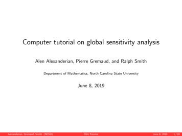
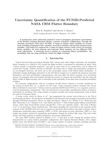
another aeroelastic CFD tool, CFL3D.15 Structural inputs to FUN3D include the list of natural frequenciesfor each mode, prescribed modal damping, the inertial force vector written in modal coordinates, and modeshapes projected onto the CFD wing surface.16Figure 2. Thickness distribution throughout the wingbox.Within FUN3D, the compressible Reynolds-averaged Navier-Stokes flow equations and the SpalartAllmaras turbulence model are solved on semi-infinite tetrahedral volume grids with prismatic elementsin the boundary layer. Two grids are considered here: a 3.1 million node mesh (coarse) and a 13.8 millionnode mesh (medium). For both grids, normal spacing of the first grid point off the vehicle is roughly y 1throughout. The surface mesh of the coarse grid is shown in Fig. 3. Finer grids are not included here, dueto the computational expense of the UQ analysis.FUN3D computations are run in three stages. First, the flow is computed over a rigid wing. This rigidsolution is then utilized as the initial condition for an unsteady flow analysis, with each modal damping ratioset to 0.99, to obtain a static aeroelastic solution. This converged solution is finally utilized as the initialcondition for a second unsteady flow analysis, with modal damping ratios set to 0 (and some prescribedmodal perturbation), to obtain a dynamic aeroelastic response history. CFD mesh deformation is obtainedvia a linear elasticity analogy.17 For the dynamic aeroelastic results, the time step size is 3·10 3 s (100steps per 3 Hz cycle), with 30 subiterations per time step. For the computational resources allocated forthis effort, roughly 15-20 aeroelastic cases (each comprising all three stages: rigid, steady, dynamic) could becompleted within a week of wall time, for the coarse CFD mesh. For the medium mesh, only 5 cases couldbe completed within a week.Figure 3. CFD surface mesh for the 3.1 million node grid.3 of 11American Institute of Aeronautics and Astronautics
C.Nonintrusive Polynomial ChaosThe method used in this work for uncertainty quantification is originally developed in Ref. 18 and will bebriefly summarized here. Some aeroelastic output of interest, Y , is assumed to be represented by a weightedcombination of basis functions written across the random variable space:Y (ξ) PXαi · Ψi (ξ)(1)i 0where ξ is a vector of random variables written in standard normal space, Ψi is the ith basis function, and αiis the corresponding weight. For the normal random variables considered here, the basis functions are a totalorder expansion of Hermite polynomials, comprising Nt P 1 (n s)!/n!/s! terms. n is the number ofrandom variables in ξ, and s is the desired order of the PCE. Further details regarding the mathematics ofthis assumed basis may be found in Refs. 18 and 19.Y values are sampled at random locations (identified through Latin Hypercube sampling) throughout therandom variable space, and then αi terms are computed by solving a least squares problem. If the numberof available samples is equal to or greater than Nt , Eq. 1 is an over-determined least squares problem. Ref.18 recommends an oversampling ratio (ratio of the number of samples to Nt ) of two. This sampling costgrows rapidly with increased n or s, however. An alternative method, used here, is to assume sparsity in thecoefficient vector α, and solve Eq. 1 as a regularized (under-determined) least squares problem. The LASSOalgorithm is used to solve this regularized problem,20 potentially at an oversampling ratio much less thanone. Tenfold cross validation is used to select the best solution of the LASSO-generated list of α vectors.21Another potential method to reduce sampling cost is to enhance the point collocation process with gradientsdY /dξ,22 though analytical aeroelastic gradients (computed via the adjoint method) are not yet available inFUN3D.Once the PCE expression of Eq. 1 is obtained, analytical expressions for the mean and standard deviationof Y are available,19 as are Sobol indices (global nonlinear sensitivity parameters).23 Alternatively, MonteCarlo sampling of the low-cost PCE may be conducted in order to obtain probability density functions(PDF), higher order moments, probabilities of failure, etc.III.Deterministic Aeroelastic ResponseFirst, the deterministic flutter boundaries of the uCRM, in terms of the matched-point dynamic pressureQ, are shown in Fig. 4 across a range of Mach numbers, for 0 and 2 angle of attack, for the coarse CFDgrid. The 15% flutter margin (assumed dive speed of 185 m/s) is also shown. Up to a Mach number of 0.8,the flutter mechanism is driven by linear physics, with a weak dependence on angle of attack. Flutter doesoccur at a margin less than 15% at Mach 0.55, and then flutter Q gradually rises above the 15% margin withincreased Mach number. Beyond Mach 0.8, mixed flow (shocks) begins to appear over the wing, causingstronger dependencies on angle of attack. At 0 , there is a pronounced flutter dip (minimum Q at Mach0.9125), followed by a sharp rise in the flutter Q. At 2 , the flutter Q is more erratic, with less of a deviationfrom the linear extrapolation. It is finally noted that the medium CFD grid provides a good match to thecoarse grid at the two selected cases in Fig. 4: 0 angle of attack, Mach 0.7 and 0.85.Flutter boundaries in Fig. 4 are found by gradually increasing Q at a given Mach number and searchingfor instabilities in the oscillatory modal coordinate output. An example of this is shown in Fig. 5 at Mach0.85 and 0 angle of attack, for four different dynamic pressures: both the static aeroelastic convergence(t 1) and the subsequent dynamic results (t 1) are shown. The mode 1 generalized coordinates (roughlycorresponding to a first bending mode) are found to be representative of the wing aeroelastic behavior as awhole, and are used to assess stability. The lowest Q value in Fig. 5 is essentially a “wind-off” condition, andthe mode vibrates at the first bending frequency (1.7 Hz), about a negative steady state deformation (due tothe self-weight forces). Higher dynamic pressures allow the aerodynamic forces to overcome the self-weightloads, leading to positive steady state deflections, and an eventual loss of dynamic stability. Using a finerQ-step than shown in the figure, the flutter point is bracketed, and the linearly-interpolated cross-over pointis plotted in Fig. 4.4 of 11American Institute of Aeronautics and Astronautics
Figure 4. Deterministic flutter boundaries of the uCRM.Figure 5. Aeroelastic time integration at Mach 0.85, 0 angle of attack.IV.Atmospheric RVs, Coarse CFD GridNext, three uncorrelated normal random variables are utilized in ξ: Mach number, dynamic pressureQ, and angle of attack. Mach number and Q are in reality dependent variables, but can be considerednumerically uncorrelated by computing the flow density and speed to ensure a matched atmospheric pointfor a given Mach/Q combination. The only system output of interest (Y ) in these results is the aeroelasticdamping of the first generalized coordinate. Specifically, the last 8 peak-to-peak logarithmic decrements inthe time history are averaged to form Y . For all cases explicitly examined, the decrements/increments arewell-converged within these last 8 cycles.Three PCEs are constructed, summarized in Table 1, expanded about the mean Mach numbers of 0.7,0.825, and 0.875. The mean angle of attack is set to 0 (1 standard deviation), and the mean Q for eachcase corresponds to the associated deterministic flutter points in Fig. 4, with a 0.04 coefficient of variation(COV). Each RV is considered to be normally distributed. For the lower mean Mach number of 0.7, alow-order PCE is found to suffice, given the near-linear aeroelastic physics seen in Fig. 4. At Mach 0.875,the stronger aerodynamic nonlinearities in the flow require a higher-ordered PCE. The statistical outputconvergence at this transonic Mach number, as a function of polynomial order s, is shown in Table 2. EachPCE in this table is built with the same 168 samples, and the mean output µY is nearly zero for all cases,as expected. For each value of s, the number of αi terms in the total order expansion (Nt ) is given, as wellas the number of terms actually utilized by the sparse LASSO solver.Probability density functions for the three PCEs in Table 1 are shown in Fig. 6, where an increase in5 of 11American Institute of Aeronautics and Astronautics
Table 1. Summary of PCEs constructed with atmospheric design variables.order s248µM ach0.70.8250.875σM ach0.0250.0250.025µQ29.10 kPa30.49 kPa30.11 kPaσQ1.16 kPa1.22 kPa1.20 kPaµAoA0.0 0.0 0.0 σAoA1.0 1.0 1.0 Table 2. Convergence of the mean µ and standard deviation σ of Y , at Mach 0.875.order s2345678full Nt1020355684120165sparse .0372087440.0366690950.037772292Mach number increases the spread in the distribution (increases σY ), and the 0.875 Mach number case showsclear skewness from the transonic flow nonlinearities. Total sobol indices (global sensitivity parameters) areshown in Fig. 6 as well, for each atmospheric random variable. Overall, the dynamic stability is most stronglyimpacted by the dynamic pressure, but this impact wanes as Mach number is increased, and angle of attackbecomes more predominant (Mach number also rises in importance, though to a much lesser degree). Theseresults echo the results of Fig. 4, where subsonic flutter is weakly dependent upon angle of attack, as opposedto transonic flutter. For truly linear aeroelasticity, there is in fact no dependence between flutter and angleof attack, given the ability to separate static and dynamic aeroelastic physics.24Figure 6. Probability distribution functions (left) and Sobol indices (right) for the three PCEs in Table 1.An additional technique, which evaluates the ability of the PCEs to emulate the sampled physics, is tocompute the flutter boundaries directly from the polynomial surrogate function in Eq. 1. This is shown inFig. 7, for comparison with the deterministic data repeated from Fig. 4. PCE-derived flutter boundariesare also shown at -2 angle of attack, for which no direct deterministic data exists. These surrogate flutterboundaries match the deterministic data points fairly well, with some exceptions. At Mach number 0.78,the 2 and -2 PCE boundaries are clearly under-fit (bias error), though the 0 model shows a smoothertransition from the Mach 0.7 PCE to the Mach 0.825 PCE. Furthermore, all of the models entirely miss thehighly nonlinear flutter boundaries at Mach 0.9, which would require a very high order polynomial to fit,particularly at 2 angle of attack.6 of 11American Institute of Aeronautics and Astronautics
It is finally noted that, according to the PCE, the response of the -2 surrogate is the most critical inFig. 7, with a flutter dip below the 15% margin line near Mach 0.88. There is no deterministic data in thisarea to verify this trend, however, and it is known from the higher angles of attack that the quality of thePCE fit deep in the transonic range is only moderate.Figure 7. Flutter boundaries predicted with PCE.V.Atmospheric RVs, Medium CFD GridThis section repeats the PCE exercise of the previous section, though with the medium CFD grid asopposed to the coarse (13.8 vs. 3.1 million nodes). This is only done for the first subsonic PCE in Table 1,expanded about Mach 0.7. Owing to the weak aeroelastic nonlinearities, the computational burden of thisPCE is fairly low; 20 samples for a converged result. Though it would be of great interest to consider a casewith mixed flow (i.e., a shock) over the wing, the computational cost for the required high-ordered PCE istoo high, at present.Good agreement in the flutter margin predicted by the two grids can be seen in Fig. 4 at Mach 0.7, withflutter-Q values of 29.10 kPa (coarse) and 29.15 kPa (medium). The logarithmic decrement of the dynamicaeroelastic response is shown in Fig. 8 for all 20 samples, as is the resulting PDF computed from the PCE. Aswith the deterministic flutter point, the statistical data also matches well between the two grids. It shouldbe noted that the comparison in Fig. 8 is not completely equitable, as the coarse-grid PCE is expandedabout a slightly different flutter point than the medium grid (29.10 vs. 29.15 kPa). Differences in resolvedflow physics also contribute to the gap in Fig. 8.Figure 8. Sampling (left) and PDF computations (right) for the two CFD grids at Mach 0.7.To this point, only the logarithmic decrement of the dynamic aeroelastic response has been considered7 of 11American Institute of Aeronautics and Astronautics
as the response output Y , for PCE generation in Eq. 1. The next result in Fig. 9 considers the pressurecoefficient at every point on the CFD surface as an uncertain variable: one second-order PCE per surfacegrid point (i.e., a multi-output case). This is only done for steady pressures, for both a rigid wing and aflexible wing. The upper contour plots in Fig. 9 show average (µY ) pressures, and in the flexible case, thesecontours are superimposed upon the average wing deformation. Given the near-symmetry of the PDFs inthese cases (seen for example in Fig. 8), average pressures will look very similar to deterministic values.The lower plots in Fig. 9 show slices of pressure data at three span stations, along with 95% confidenceintervals (computed from σY ). For the rigid wing, the dynamic pressure RV is of minor importance relativeto Mach number and angle of attack. Given the matched point atmospheric conditions, Q of a rigid wingwill alter the Reynolds number and the flow temperature, but these dependencies upon Cp are minor. Forthe flexible wing, the Q RV is of course a strong driver due to the aeroelastic re-distribution of loads. Wingtwist in Fig. 9 about the elastic axis is small, but bending deformations are larger, and positive bending ofa swept wing will decrease the effective angle of attack.24 This shedding of outboard airloads is clearly seenin Fig. 9.Figure 9. Average rigid and flexible static pressure distributions (top row), and pressure slices with 95%confidence intervals (bottom rows).As noted, there is no shock in the flow data of Fig. 9, at Mach 0.7. Peak uncertainties, implied by theconfidence intervals (computed via µY ), therefore occur near the leading edge (as opposed to a transoniccondition, where uncertainties would presumably be largest near the shock) of the upper surface. Overalluncertainty levels are higher for the rigid wing than for the flexible wing. This is perhaps surprising giventhe random fluctuations in wing shape that will be found in the flexible case, and also given that one of thethree RVs (Q) has almost no impact on the output uncertainty of the rigid wing. A likely cause for thisresult is the load-alleviating nature of the swept flexible wing, which can passively adapt to fluctuations inMach, angle of attack, and Q, whereas the rigid wing cannot. The inclusion of trim loads, which are not8 of 11American Institute of Aeronautics and Astronautics
considered here (i.e., CL is not the same between the rigid and flexible cases), may demonstrate a more evenlevel of uncertainty between the rigid and flexible wings.VI.Atmospheric, Structural, and Inertial RVs, Coarse CFD GridThe final section in this paper reverts back to the coarse CFD mesh, but expands the list of randomvariables. These include: 1) Mach number, 2) angle of attack, 3) dynamic pressure, 4) inboard skin thickness,5) outboard skin thickness, 6) inboard spar thickness, 7) outboard spar thickness, 8) rib thickness, 9) leadingedge mass, 10) trailing edge mass, and 11) engine mass. Each random variable is normally-distributed, anddefined as follows: Atmospheric RVs (Mach number, angle of attack, dynamic pressure): these are repeated from Table 1,using the expansion about Mach 0.7. Structural thickness RVs (inboard and outboard skin thickness, inboard and outboard spar thickness,and rib thickness): the mean values for these variables are the patchwise distributions seen in Fig. 2,with a 0.04 COV. For a given RV (e.g., inboard spar thickness), each of the patchwise values in thatset are assumed to randomly scale up or down in tandem, perfectly correlated. In reality, each patchwill have its own probability distribution with varying degrees of correlation to adjacent patches, butthe current assumption is required to keep the number of RVs low. Inertial RVs (leading edge, trailing edge, and engine lumped mass): as above, the mean values (µ) areset to the deterministic values used previously (graphically shown in Fig. 1, with a total engine massof 5,200 kg, total leading edge mass of 1,200 kg, and trailing edge mass of 2,470 kg), with a 0.04 COV.Each lumped mass attached to a given RV scales up or down in tandem.The structural sizing RVs can impact both elastic and inertial properties of the wing, with inboard thicknesshaving a greater impact on wing stiffness, and outboard thickness a greater impact on inertial properties.The lumped inertial mass RVs have no stiffness contribution. In order to properly account for the aeroelastictrends due to structural and inertial parameterizations, the NASTRAN model is rerun for each sample (tocompute vibration frequencies, mode shapes, and self-weight terms), prior to exercising FUN3D.These eleven RVs are characterized with a 2nd -order PCE built upon 80 samples. Though not shownhere, PCE-based statistical output from a 40-sample model compares well to the 80-sample model, suggestingadequate convergence. Sobol indices for three outputs metrics (computed from three separate PCEs) areshown in Fig. 10: the vibration frequency of the first bending mode (wind-off), the static aeroelastic tipdeflection, and the dynamic aeroelastic logarithmic decrement. The bending frequency metric is not anaeroelastic quantity, and so the atmospheric RVs have no contribution. Inboard skin thickness is the maindriver here, and the outboard inertial properties (leading/trailing edge lumped mass, outboard skin thickness)have a secondary role. It is important to note that the first bending mode does not typically become thefluttering mode (in wind-on conditions) for these cases. The fluttering mode is usually mode three; a torsionalmode with a high degree of engine pitch.Figure 10. Sobol indices for various response outputs: first bending frequency (wind-off ), static aeroelastictip deformation, and dynamic aeroelastic logarithmic decrement.The statistical behavior of the second metric in Fig. 10, the static aeroelastic wingtip deflection (cf.,seen graphically in Fig. 9), is overwhelmingly driven by the angle of attack RV. In theory, all eleven RVs9 of 11American Institute of Aeronautics and Astronautics
will contribute to static aeroelastic deflections through changes in aerodynamic, inertial, or elastic forcebalancing. The uncertainties in angle of attack, however, are extremely large, with a standard deviation of1 . For transonic flutter, this range of uncertainty places the angle of attack RV on roughly the same levelof importance as the other RVs. For static aeroelastic effects, however, such a distribution monopolizes theprobabilistic response, in comparison to a 0.04 COV on skin thickness (for example).The final metric in Fig. 10, the dynamic aeroelastic logarithmic decrement, is computed as discussedin the previous sections. This metric has a more even spread of Sobol indices, with dynamic pressure andthe engine mass constituting the main drivers (as noted, the flutter mode shape is characterized by enginepitch), and structural thicknesses playing a secondary role. Angle of attack in this case has a very smallSobol index owing to the subsonic flow conditions (Mach 0.7), as also seen in Fig. 6.For this eleven-RV case, a relationship between flutter margin and flutter probability is shown in Fig. 11,in the form of a cumulative distribution function. For the commonly-considered 15% flutter margin (shownin Fig. 4 and Fig. 7), the probability that the wing will flutter within this margin, at Mach 0.7, is 0.202.Referencing back to the Introduction of this paper, the more important question is: what is the probabilitythat the wing will flutter within the flight envelope (i.e., the probability that the flutter margin will be lessthan zero)? As noted, a long-term goal is to replace the 15% flutter margin with a UQ-driven Pf threshold.As seen on the log-scale plot of Fig. 11, the current PCE does not have enough information within the tailof the failure function to accurately compute this 0%-margin Pf value. A Monte Carlo sampling of the PCEcomputes Pf as 4 · 10 7 , though a simple moment projection19 estimates Pf as 2.2 · 10 8 .Figure 11. Cumulative distribution function of flutter probability vs. flutter margin (linear scale on left, logscale on right).VII.ConclusionThis work has conducted an uncertainty quantification analysis of the Common Research Model with aflexible wingbox, using FUN3D and NASTRAN. The main output metric of interest is the damping characterof the dynamic aeroelastic wing response (logarithmic decrement), due to some perturbation: this metric willbe exactly zero at the flutter point. Secondary metrics include steady pressures, structural displacements,and structural vibration frequencies. A nonintrusive sparse PCE is used to propagate uncertainties throughthe aeroelastic model, with atmospheric, structural, and inertial RVs all considered. Finally, two CFDmeshes are included in this work: a coarse grid (3.1 million nodes) and a medium grid (13.8 million nodes).For fully subsonic flow conditions, the flutter mechanism is essentially linear. Computationally inexpensive low-ordered PCEs provide accurate representations of the statistical aeroelastic output. Relatively largenumbers of random variables can be included in these models, and it is expected that the eventual inclusion ofaeroelastic adjoint-based sensitivities in FUN3D can be used to drive the sampling cost down even further.22For transonic flows, on the other hand, the CRM exhibits strong nonlinearities, with rapid undulations inthe flutter margin across dynamic pressures. The polynomial-based surrogate PCE does not perform as wellhere, with larger sampling costs needed to approximate the aggressive curvature in the random parameterspace. Sparse approximations12 can be used to temper costs, but plotting the deterministic transonic fluttermargins alongside the PCE-derived margins still reveals gaps between the two.10 of 11American Institute of Aeronautics and Astronautics
The ultimate goal of this work is to replace the typical 15% flutter margin, frequently used in design work,with a rigorous failure probability threshold.3 Beyond the typical challenges associated with reliability-basedUQ (i.e., how to quantify input uncertainties, how to ascertain an appropriate Pf constraint boundary, howto propagate uncert
the CRM are modeled aerodynamically, but are assumed rigid. The engine is modeled inertially, but not aerodynamically. B. Aeroelastic Analysis The nominal sti ness properties of the uCRM wingbox, taken from Ref.14, are shown in Fig.2, in terms of the shell thickness, smeared sti ener thickness, and smeared sti ener height. A NASTRAN nite element