WIXLIB

1444A. Delorme et al. / NeuroImage 34 (2007) 1443–1449to be an efficient method for separating distinct artifactual processes including eye blink, muscle and electrical artifacts (Barbatiet al., 2004; Delorme et al., 2001; Iriarte et al., 2003; James andGibson, 2003; Joyce et al., 2004; Jung et al., 2000b; Tran et al.,2004; Urrestarazu et al., 2004; Zhukov et al., 2000). Althoughseveral ICA algorithms in different implementations have beenused to separate artifacts from EEG and MEG data, they all can bederived from related mathematical principles (Lee et al., 2000).While ICA is now considered an important technique for detectingartifacts, there are still few quantitative measures of the advantagefor artifact detection that is gained from ICA decomposition.Here we develop a framework for comparing artifact detectionmethods and use it to determine whether preprocessing EEG datausing ICA can help in detecting brief data epochs that containartifacts. We first apply a set of statistical and spectral analysismethods to detect artifacts in the raw data, optimizing a freeparameter for each method so as to optimally detect knownartifactual data epochs. Then, we apply the same procedure to thedata decomposed using ICA. Finally, we quantitatively compareresults of these artifact detection methods applied either to raw orto ICA-preprocessed data.Methods of artifact detectionWe compared five different methods for detecting trialscontaining artifacts (Barbati et al., 2004; Delorme et al., 2001):1. Extreme values. First, we used standard thresholding ofpotential values. Here, data trials were labeled as artifactual if theabsolute value of any data point in the trial exceeded a fixedthreshold. This method is currently the most widely used artifactdetection method in the EEG community. It is most effective fordetecting gross eye blinks or eye movement artifacts.2. Linear trends. Marked linear trends at one electrode typicallyindicate transient recording-induced current drifts. To detect suchevents, we measured the goodness of fit of EEG activity to anoblique straight line within data epochs’ length. We then eithermarked or not the data trial depending on the minimum slope ofthis straight line and its goodness to fit (in terms of r2).3. Data improbability. Most artifacts have “unusual” timecourses, e.g., they appear as transient, ‘odd’ or unexpected eventsand may be so identified by the outlying values of their statisticsrelative to normal brain activity. We tested the use of the jointprobability of the observed distribution of data values and thekurtosis of the data value distribution for detecting such artifacts.To estimate the relative probability of each trial from the data, wefirst computed the observed probability density function (De) ofdata values over all trials for each electrode e (over 4165 equallyspaced bins, giving a total of 20,285 values per channel orcomponent activity). Each data sample point was thus associatedwith a probability. Then, we computed the joint log probability Je(i) of the activity values (Ai) in each data trial i and electrode e by!YJe ðiÞ ¼ logpDe ðxÞð1ÞxaAiwhere pDe (x) is the probability of observing the value x in theprobability distribution De of activity at electrode e. We used thejoint log probability for more effective graphic presentation ofvery low joint probability values. The joint probability wascomputed for every data trial at each electrode or independentcomponent.4. Kurtosis. We used a second measure to detect unusually‘peaked’ distributions of potential values — the kurtosis (K) of theactivity values in each trial.K ¼ m4 3m22ð2Þmn ¼ Efðx m1 Þn gð3Þwhere mn are the nth central moments of all activity values in thetrial (m1 their mean), and E an expectation function (here, theaverage). If all activity values are similar, or the values alternatebetween two or more extremes, the kurtosis will be highlynegative. Again, this type of activity is not typical of brain EEGsignals. Strong negative kurtosis values usually reflect AC(alternating current) or DC (direct current) artifacts, for example,those induced by screen currents, strong induced line noise fromelectrical machinery, lighting fixtures or loose electrode contacts. Ifthe kurtosis is highly positive, the activity distribution is highlypeaked (usually around zero) with infrequent appearance ofextreme values, and the identified data are likely to contain anartifact. For example, starting with a signal (random time series)having low negative kurtosis and adding a transient 10-foldincrease in signal amplitude lasting for only a total of 0.001% ofthe data length (modeling for example the presence of an electricalartifact) may be sufficient to invert the sign of the kurtosis andproduce a positive kurtosis value. Eye blink artifacts, as forexample extracted from scalp EEG data by ICA, also haverelatively high kurtosis.Before defining detection thresholds for joint probability and forkurtosis, we first normalized these measures to have zero mean andunit standard deviation. We were thus able to define (z) thresholds interms of standard deviations from expected mean values.5. Spectral pattern. Finally, some EEG artifacts have specificactivity and scalp topographies that are more easily identifiable inthe frequency domain. For instance, temporal muscle activationstypically induce relatively strong 20–60 Hz activity at temporalelectrodes, while saccadic eye blinks produce unusually strong(1–3 Hz) low frequency activity at frontal electrodes. To detect theseartifacts, we computed the Slepian multitaper spectrum (Thomson,1982) for each single trial and each single channel, using Matlabpmtm function defaults (4 orthogonal tapers; FFT length of 1024data points for each data epoch). The main advantage of using multitaper over standard spectral methods is that, for rhythmic activity inthe data, the signal/noise ratio may be lower (Thomson, 1982). Toreveal deviations from baseline, we then subtracted the epoch meanspectrum for each channel and finally applied maximum thresholding to the resulting trial spectral estimate.Software routines for performing the artifact detection methodsdescribed above are available within the EEGLAB toolbox(Delorme and Makeig, 2004).Data simulationTo test and optimize the artifact detection process, we usedevent-related EEG data from a ‘Go/Nogo’ visual categorizationtask (Delorme et al., 2004). EEG was recorded at a 1000 Hzsampling rate using a 32-electrode scalp montage with all channelsreferenced to the vertex electrode (Cz). The montage did notinclude specific eye artifact channels, but did include channels forelectrodes located above the eyes (FPz; FP1, FP2). Responses totarget and non-target stimuli presented about every 2 s were

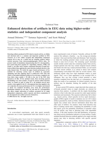
A. Delorme et al. / NeuroImage 34 (2007) 1443–1449recorded for each subject. Data epochs were extracted surroundingeach stimulus, extending from 100 before to 600 ms after stimulusonsets. The mean value in the pre-stimulus baseline ( 100 to 0 ms)was subtracted from each individual epoch. Data were then prunedof noticeable eye and muscle artifacts by careful visual inspection(AD), resulting in 119 “clean” data epochs.We then simulated five types of artifacts (Fig. 1):(1) We modeled eye blink time courses using random noiseband-pass filtered (FIR) between 1 and 3 Hz. Eye blinks havestereotyped scalp topographies that can be isolated using ICA(Jung et al., 2000b). To obtain topographical maps for thesesimulated eye blinks, we applied ICA decomposition to datafrom another subject and visually identified an eye blinkcomponent by its time course and scalp topography (highgains on the most frontal electrodes; small gains everywhereelse). We used a blink scalp topography from another subjectto ensure that the simulated data and the real data wereseparable and independent of each other.(2) We modeled temporal muscle artifacts using random noiseband-pass filtered (FIR) between 20 and 60 Hz andmultiplied by a typical muscle scalp map, again isolated byICA from another subject (high gains at a few temporalelectrodes and near zero gains for other electrodes).(3) We then modeled electrical shift artifacts by implementingdiscontinuities at one randomly selected data channel.(4) We also modeled unfiltered white noise at another randomlyselected data channel.(5) Finally, we modeled linear trends (with randomly selectedslopes from 100 to 300 μV per epoch at the lowest level ofnoise) at another randomly selected data channel.In the test data depicted above, each data channel could onlyhave one type of artifact, excepting the first two artifact types (eyeand muscles), which projected with varying strengths to all theelectrodes. We took care that the randomly selected channels foreach artifact type differed from each other and did not coincidewith channels where the two first topographical artifacts hadmaximum amplitude.Since our goal was to test the sensitivity of each method fordetecting artifacts, we varied simulated artifact amplitude to findthe smallest artifacts that each method in the “Methods of artifact1445detection” section could detect. Artifacts at the smallest amplitudelevel ( 50 dB) were so small that none of the methods was able todetect them. For each artifact type, amplitude was graduallyincreased from 50 dB to 0 dB. To compute signal to noise ratio(SNR; i.e., artifact to background brain EEG signal ratio), wedivided the spectrum of each type of artifact (not mixed yet withdata) at each frequency by the data spectrum at the same frequency.We then found the frequency with the largest SNR and converted itto dB scale (10 * log10(SNR)). Prior to computing SNR for the firsttwo (topographic) artifacts, we scaled their amplitudes by thehighest channel gain in the applied scalp map.Automatic artifact detectionSince we knew which data trials contained simulated artifacts,for each type of artifact, we could determine the most efficientartifact detection method. For each method, we chose one freeparameter which we optimized to estimate an upper bound on theability of the method to detect artifacts of the given type.We assumed voltage thresholds to be symmetrical, so only oneparameter had to be optimized in the standard thresholdingmethod. Linear trend detection had two parameters (minimumslope and goodness of fit). We set the slope to be equal or higherthan the minimal artifactual slope at the maximum level of noise(0.5 μV/700 ms) and then optimized the goodness-of-fit parameter.Since this was time consuming and was specifically aimed atdetecting trends, we applied this method only to detecting lineartrend artifacts and not other types of artifact. For the probabilityand kurtosis methods, we optimized the z threshold. Finally, forthe spectral measure, we optimized the dB limits independentlyfor three frequency bands (0 to 3 Hz, 20 to 60 Hz and 60 to125 Hz) and then used the frequency band that returned the bestresults.For each parameter, the optimization procedure minimized thetotal number of trials misclassified (misses plus false alarms). Toreduce the computational load, we used a procedure thatrecursively divided its value range until a minimum was reached.More powerful nonlinear optimization methods we considered,using Matlab Nelder–Mead multidimensional unconstrained nonlinear minimization, proved computationally infeasible. Weattempted to design an algorithm requiring the least number ofiterations while minimizing the risk of falling into local minima. ToFig. 1. (A) Types of simulated artifacts (top panels) introduced into actual EEG data epochs (bottom panel ordinate, 50 μV). Ticks indicate 700-ms epochboundaries. (B) Simulated data obtained by adding the simulated artifacts (A) to the EEG data. Artifacts shown here were the largest simulated (0 dB); thesmallest were more than 100,000 times smaller ( 50 dB).

1446A. Delorme et al. / NeuroImage 34 (2007) 1443–1449perform the optimization, we thus divided the parameter intervalrange into 10 equally spaced intervals and evaluated the number ofcorrectly classified trials at these points. We located the two valuessurrounding local minima and created a new interval. Then, we ranthe procedure recursively three times, repetitively dividing thenewly created value range into 10 intervals and counting correctlyclassified trials, thus obtaining the ‘optimal’ parameters for eachdetection algorithm.ICA-based artifact detectionICA separates EEG processes whose time waveforms aremaximally independent of each other. The separated processes maybe generated either within the brain or outside it. For instance, eyeblinks and muscle activities produce ICA components with specificactivity patterns and component maps (Jung et al., 2000b; Makeiget al., 1997). However, scalp EEG activity as recorded at differentelectrodes is highly correlated and thus contains much redundantinformation. Furthermore, several artifacts might project to overlapping sets of electrodes. Thus, it would be useful to isolate andmeasure the overlapping projections of the artifacts to all theelectrodes and this is what ICA does (Jung et al., 2000a; Makeig etal., 1996).To build intuition about how ICA works, one might imaginean n-electrode recording array as an n-dimensional space. Therecorded signals can be projected into a more relevant coordinateframe than the single-electrode space: e.g., the independentcomponent space. In this new coordinate frame, the projections ofthe data on each basis vector – i.e., the independent components –are maximally independent of each other. Intuitively, by assessingthe statistical properties of the data in this space, we might be ableto isolate and remove the artifacts more easily and efficiently.Multiplication of the scalp data, X, by the unmixing matrix, W,found for example by Infomax ICA represents a linear change ofcoordinates from the electrode space to the independent componentspace, orS ¼ WTXð4Þwhere S is the ‘activation’ matrix of the components across time.Each component is a linear weighted sum of the activity of anindependent source process projecting to all of the electrodes. Eachrow of the unmixing matrix W that extracts each componentactivity time course may be seen as a spatial filter for a distinctiveactivity pattern in the data. Each independent componentcomprises an activation time course plus an associated scalp map(the corresponding column of W 1) that gives the relativeprojection strengths (and polarities) of the component to each ofthe electrodes.All the artifact detection methods described in the previoussection were also applied to raw potential values decomposedusing different ICA algorithms. In this study, we used three ICAalgorithms most often used to date to process EEG data: InfomaxICA, SOBI and FastICA. These ICA algorithms have the sameoverall goal (Lee et al., 2000) and generally produce near-identicalresults when applied to idealized source mixtures. The approach ofeach algorithm to estimating independence is different: Infomaxemploys a parametric approach to estimate the componentprobability distributions (Bell and Sejnowski, 1995), whereasFastICA maximizes the neg-entropy of the component distributions(Hyvarinen and Oja, 2000). SOBI is a second-order method thatrequires and takes advantage of temporal correlations in the sourceactivities (Belouchrani and Cichocki, 2000). Results produced bythese algorithms may differ when the component activities are notfar from Gaussian or are not independent.For Infomax, we used default parameters as implemented in therunica function of the EEGLAB toolbox (Delorme and Makeig,2004). These involved pre-sphering of the data and stoppingtraining when weight change was less than 10 6. Since extendedInfomax ICA decompositions revealed that the EEG data did notcontain any sub-Gaussian component, we here used the nonextended version of Infomax for somewhat faster computation(sub-Gaussian components of EEG data include single-frequencyline noise, not simulated here). Since we were processing dataepochs rather than continuous data, we slightly modified the SOBIalgorithm (Belouchrani and Cichocki, 2000) so that data covariance matrices for different time delays were computed for eachepoch then averaged over data epochs. This modified version ofthe SOBI algorithm has currently been made available for testingin the EEGLAB toolbox (Delorme and Makeig, 2004). Whenrunning SOBI, we set to 100 the number of correlation matrices atdifferent time delays (Akaysha Tang, personal communication).For the FastICA algorithm (Hyvarinen and Oja, 2000), we forcedthe decomposition to estimate all components in parallel (“symmetric” approach for version 2.1 of the FastICA algorithmavailable on the Internet), setting believed to be suitable for EEGdata analysis (Aapo Hyvärinen, personal communication). Sincewe could not determine which component contained relevantartifacts, for each artifact type, each detection method was appliedto all components and the single component returning the bestresults was used in the detection process.Altogether, we generated a total of 20 datasets with differentartifact and noise instantiations and then used a Linux cluster of 36processors (1.4 GHz or faster) to optimize parameters for eachdetection method and each dataset. The results presented hererequired about 24 h of computation on this cluster.ResultsResults for each detection method and each artifact type arepresented in Fig. 2, which shows results for one artifact type ineach row and one detection method in each column. Applied eitherto the raw data or to ICA component activities, the frequencythresholding method performed the best overall; the joint probability method was second best, and standard thresholding third.Kurtosis thresholding performed the poorest, though it was partlysuccessful in detecting large discontinuity and trend artifacts.Finally, the trend detection method was the most efficient fordetecting linear trends in the data, although nearly equal performance was achieved using the frequency thresholding method(1–3 Hz band).However, one has to balance the performance advantageagainst the speed of computation. Here, simple thresholding wasfastest, while the joint probability was 4 times slower, kurtosisrejection was 8 times slower, trend rejection was about 25 timesslower, and spectral rejection was about 120 times slower.However, for all detection methods, the measure of interest (jointprobability, kurtosis, slope, or spectrum) does not need to becomputed several times. Once a measure has been computed,simple thresholding may be applied repeatedly to obtain optimalresults (see Methods of artifact detection). The EEGLAB routinesthat implement these detection methods use this strategy (Delormeand Makeig, 2004).

A. Delorme et al. / NeuroImage 34 (2007) 1443–14491447Fig. 2. Artifact detection performance (artifacts detected minus non-detected artifacts, divided by the total number of artifacts) by five methods (columns) appliedto detection of the five types of simulated artifacts (rows, cf. Fig. 1) at a range of amplitudes (0 to 50 dB relative to the EEG). Linear trend detection (far right)was only used to detect trend artifacts. Black traces: the five methods were first applied optimally to the best single-channel data for each artifact type. Graytraces: the same methods were then applied to the best single independent components computed from the data by Infomax ICA. Vertical error bars show 1standard deviation in performance across 20 replications. Overall, for artifacts less than 40 dB below the EEG in strength spectral thresholding methods (right)performed best, and all detection methods performed better when applied to the independent component data.In Fig. 3, we then attempted to compare the performance ofartifact detection applied to the raw data and to the same datapreprocessed using ICA. To do so, we only considered thefrequency thresholding method since it outperformed mostmethods for all types of artifacts. Since the performance trend,as artifact size decreased, was different for each artifact type, wenormalized each performance curve to the logistic functionbefore averaging. To do so, we fitted each performance curveobtained from simulated data with a sigmoid function byoptimizing its slope and horizontal offset. We then normalizedthe observed data points on each curve so they would lie on asigmoid curve centered on 0 with slope 1. We applied the sametransformation to the ICA results using the normalizationparameters obtained from the simulated data (this explains whystandard deviations were larger for the ICA results than for rawdata results). Finally, we plot the mean normalized performancecurves for the raw and ICA-separated data for all three ICAalgorithms we tested—Infomax, SOBI and FastICA (see Methodsof artifact detection). We expected that frequency thresholdingwould be more efficient when applied to data preprocessed byany of the tested ICA algorithms than when applied to raw data.This is indeed what we observed (Fig. 3). Data preprocessing byICA led to a 10–20% increase in artifact detection performancefor all the three ICA algorithms tested. Detection performancewas best using Infomax ICA, approaching two standarddeviations above raw data mean detection performance (shadedarea in Fig. 3).DiscussionWe have shown that optimally applying spectral methods toidentify artifacts in 32-channel EEG data epochs allowed morereliable detection of smaller artifacts than optimally applying thesame thresholding methods to the scalp channel data itself.Preprocessing the data using ICA allows more effective artifactdetection. However, it should be noted that the frequencythresholding methods are as efficient at detecting muscle artifactin either the raw or ICA-decomposed data. For this type ofartifact, ICA decomposition does not seem to improve artifactdetection.In our simulated data, mixing of artifacts with data wasperfectly linear. Might this not be the case for real data? In fact,instantaneous mixing via EEG volume conduction of artifacts andEEG processes is linear. By Ohm’s law, externally imposedelectrical artifacts (DC trends, discontinuities, white noise) alsomix linearly with EEG data at scalp electrodes. On this basis, atleast, linear ICA decomposition algorithms are not inappropriatefor separating artifacts from other data processes. On the otherhand, these simulations may have disadvantaged the ICA approachsince, for example, the simulated muscle artifacts may have been

1448A. Delorme et al. / NeuroImage 34 (2007) 1443–1449Fig. 3. Comparison of artifact detection performance by spectral thresholding methods applied first to the raw channel data (gray band) and then to the same dataafter decomposition by three ICA algorithms (solid and dashed traces). Detection performance for each artifact type across a 50-dB amplitude range was fitted toa logistic function; these functions were then fit to each other and averaged across the six artifact types. The artifact strength unit (abscissa) thus indicates a 1-dBto 3-dB amplitude step, depending on artifact type. Shaded areas: performance range (boundaries, 1 SD) for the scalp channel data. Solid and dashed traces:performance range for the independent component decomposition of the same data. For all but the largest artifacts (left), detection performance using the ICAcomponents was 10–20% better than using the scalp channel data.mixed with some actual low-level muscle activity in the ‘clean’EEG. This might explain why muscle artifact detection applied tothe ICA decompositions did not strongly outperform artifactdetection applied to the raw data.Here we optimized each measure threshold based on our‘ground-truth’ knowledge of the simulated data. Note thatthreshold optimization might be of most benefit when appliedto the raw channel data, where frequency domain thresholds mustbe finely tuned to best separate artifacts from the backgroundnoise. Optimal tuning of frequency-domain thresholds for ICAcomponent activities might be less important in the (typical) casein which ICA largely isolates stereotyped eye blink, muscle, heartand line noise artifacts to a single ICA component.ICA assumptionsFirst, several major assumptions of ICA seem to be fulfilledin the case of EEG recordings. As mentioned previously, a firstassumption is that the ICA component projections are summedlinearly at scalp electrodes. A second assumption is that sourcesare independent. This is not strictly realistic but even if theappearance of artifacts might be related to brain activity –muscle contractions, for example, triggered by activity in themotor cortex – the time courses of the resulting artifacts and thetriggering brain events should typically be

9500 Gilman Drive, La Jolla, CA 92093-0961, USA Received 17 February 2006; revised 21 October 2006; accepted 2 November 2006 Available online 26 December 2006 Detecting artifacts produced in EEG data by muscle activity, eye blinks and electrical noise is a common and important problem in EEG research. It is now widely accepted that independent .