WIXLIB

IEEE TRANSACTIONS ON KNOWLEDGE AND DATA ENGINEERING participation index E .#C 5 m j of a co-location C9 7j op q "! P]"EKL .#C 5 . The participationis nindex is used as the measure of prevalence of a co-location for two reasons. First, the participationindex is closely related to the cross- function [16], [17] which is often used as a statistical measure of" #" be exploited for computational efficiency. The participation ratio can be computed as rhsut1vxw y{z} x B w y]z} x y{z y{z vF t v w w ,where is the relational projection operation with duplication elimination. For example, in Figure 2, row ]\T @ ]\ G A @ ?Z XWY @ ?Z . Only two (@ ]\ and @ ?Z ) outinstances of co-location @6 are A N aZ .of five instances of spatial feature @ participate in co-location @6 . So EKLY. @6 @ 5 Similarly, EKLY. @6 5 is 0.75. The participation index E . @6 N5 min(0.75, 0.4) 0.4. The conditional probability C E%.iC , C 5 of a co-location rule C , C is the fraction of row instances" " i b of C ) -reachable to some row instance of C . It is computed as w r v y{z} x B w y{z} x B y{y{z z v{v{ w w , where is therelational projection operation with duplication elimination. For example, in the co-location rule , 0" " b in Figure 2, the conditional probability of this rule is equal to w rh v y{z} x B w y]z} x y{z y]z v{ #v{ 1 w V3interaction among pairs of spatial features. Second, it also possesses an anti-monotone property which canIII. C O - LOCATION M INING A LGORITHMIn this section, we introduce a co-location mining algorithm. Note that the prevalence measure used inFigure 3 is the participation index and that a co-location pattern is prevalent if the values of its participationindex is above a user specified threshold.As shown in Figure 3, the algorithm takes a set c of spatial event types, a set of event instances,user-defined functions representing spatial neighborhood relationships as well as thresholds for interestmeasures, i.e. prevalence and conditional probability. The algorithm outputs a set of prevalent co-locationrules with the values of the interest measures above the user defined thresholds.The initialization steps (i.e., steps 1 and 2 in Figure 3) assign starting values to various data-structuresused in the algorithm. We note that the value of the participation index is 1 for all co-locations of size1. In other words, all co-locations of size 1 are prevalent and there is no need for either the computationof a prevalence measure or prevalence-based filtering. Thus, the set0of candidate co-locations of size

IEEE TRANSACTIONS ON KNOWLEDGE AND DATA ENGINEERING Input:8 (a) Event-ID, Event-Type, Location in Space representing a set of events(b) Set ofboolean spatial event types(c) Spatial relationship(d) Minimum prevalence threshold and conditional probability threshold .Note that participation index is the measure of prevalence.Output:A set of co-locations with prevalence and conditional probability values greaterthan user-specified minimum prevalence and conditional probability thresholds.Variables: k: co-location size: set of candidate size- co-locations: set of table instances of co-locations in: set of prevalent size- co-locations: set of co-location rules of size: set of coarse-level table instances of size-k co-locations inSteps:1.Co-location size;;; generate table instance( , E);2.3.if (fmul TRUE) then4. generate table instance( ,multi event( ));to be empty for;5.Initialize data structure6.while(not emptyand) do7. generate candidate colocation( , k);8.if(fmul TRUE) then9. multi resolution pruning( ,,multi rel( ));10. generate table instance( ,, , ); select prevalent colocation( ,,);11.12. generate colocation rule( ,,);13.; g g «ª % % g % h h µ g ¶ ¶ ¶ g ¶Y ¶Y g g¶ ¶ ¶Y · ¶Y ¶ ¶Y ¡ º¹ ª return union( º» ¼ ¼ ¼V ¶ );14.15.Fig. 3. ¡ § ª ² ³ Overview of the Algorithms1 as well as the setThe set ½of prevalent co-locations of size 1 are initialized to c of table instances of size 1 co-location is created by sorting the set , the set of event types.of event instances byevent types. If a multi-resolution pruning step is desired, the set of events are discretized into coarse levelinstances. The set 0of coarse-level table instances of size 1 co-locations is generated by sorting thecoarse-level event instances by event types.The proposed algorithms for mining co-location rules iteratively perform four basic tasks, namelygeneration of candidate co-locations, generation of table instances of candidate co-locations, pruning, andgeneration of co-location rules. These tasks are carried out inside a loop iterating over the size of theco-locations. Iterations start with size 2 since our definition of prevalence measure allows no pruning forco-locations of size 1.

IEEE TRANSACTIONS ON KNOWLEDGE AND DATA ENGINEERING9A. Generation of Candidate Co-locationsWe could rely on a combinatorial approach and useco-locations from size¿S EKL M L ¾ U P[2] to generate size¿;À \candidateprevalent co-locations.½ j , the set of all prevalent size ¿ co-locations. The functionÁ M 1 P step, we join ½ j with ½ j . This step is specified in a SQL-like syntaxworks as follows. First, in the VThe apriori-gen function takes as argumentas follows:ÅÓVÃcÅ ÂqÃ#ÓVÅÄ Ã6 Ç !Æ Æ!Æ Å Ã Ç Ã Å Æ ÈuÉ ÊiËFÌ Í]ÎNÏ!ÈuÉ Î Ð!Ì ÍbÑ Ç Æ ÈuÉ ÊÒË{Ì Í]ÎNÏ!ÈuÉ ÎkÐ!Ì ÍbÑÅ Ç Æ Æ!Æ Å Ã Ô Ç Ã Ô Å Ã/ÕÖÇ ÃP 0 j such that some size ¿cl \Next, in the EKLk U step, we delete all co-locations Cjin ½ :insert intoselect .f , .f , , .f , .f ,from,where .f .f ,, .f .f,,.f.f ;ÙÏ Ø Ü Ú2Ó Ã Û ÐpØ ÂqÃ#Ä Ï Ð Ð [ Ã1ħ " of ½ j refers to the feature of co-locations in table ½ jNote that the columnjtable instance id of table ½ refers to table instances of appropriate co-locations.forall co-locationdoforall sizesubsetsofdoif () then deletefromsubset ofCis not;and the columnB. Generation of Table Instances of Candidate Co-locationsComputation for generating sizequery:ÅÐ Ý ÅÇ¿ À \candidate co-locations can be expressed as the following join Æ Æ!Æ ÅÝÐp Ø ÂqÅ Ã#Ä Çà ØßÞ Å Ð Æ!!Æ Æ ÅÐ Ãforall co-locationinsert into/*is the table instance of co-location*/select .instance , .instance ,, .instance , .instancefrom .table instance id, .table instance idwhere .instance .instance ,, .instance .instance.instance );end;Ã Ô ÅÃ, ( .instance ,0 j}àp and table instances of the size ¿ prevalent ?R Sed f U 1P Q R STP C U á[ and C ?R Sed f U !PgQ R S P ChU áV specifyco-locations as arguments and works as follows: CThe query takes the size¿ À \à ÇÇÃ Ô Çcandidate co-location set

IEEE TRANSACTIONS ON KNOWLEDGE AND DATA ENGINEERINGthe table instances of the two co-locations joined inS EKL M L ¾ U P10Cto produce . Here, a sort-merge joinis preferred because the table instances of each iteration can be kept sorted for the next iteration. Thisfollows from a similar property of apriori-gen [2]. Sort order is based on an ordering of the set of featuretypes to order feature types in a co-location to form the sort-field. Finally, all co-locations with emptytable instances will be eliminated from0 j àp .The join computation for generating table instances has two constraints, a spatial neighbor relationshipE a 1PgQ R STP ChU jT}âm a 1PgQ R STP ChU j 5 ) ) and a combinatorial distinct event-type constraint (E ? 1P Q R STP C U âm ? !PgQ R S P ChU h E a 1P Q R STP C U j ãK âe ? 1P Q R STP C U j ãK ). We examine three strategies for computing this join:constraint ((a geometric strategy, a combinatorial strategy, and a hybrid strategy. These are described in forthcomingsubsections. Exploration of other join strategies is beyond the scope of this paper but we may exploresuch strategies in future work.Geometric Approach: The geometric approach can be implemented by neighborhood relationship-basedspatial joins of table instances of prevalent co-locations of size¿with table instance sets of prevalentco-locations of size 1. In practice, spatial join operations are divided into a filter step and a refinementstep [18] to efficiently process complex spatial data types such as point collections in a row instance. Inthe filter step, the spatial objects are represented by simpler approximations such as the MBR - MinimumBounding Rectangle. There are several well-known algorithms, such as plane sweep [3], space partition[11] and tree matching [13], which can then be used for computing the spatial join of MBRs using theoverlap relationship; the answers from this test form the candidate solution set. In the refinement step,the exact geometry of each element from the candidate set and the exact spatial predicates are examinedalong with the combinatorial predicate to obtain the final result.Combinatorial Approach: The combinatorial join predicate (i.e.E a 1PgQ R STP ChU âm a 1PgQ R STP ChU h E a 1PgQ R STP ChU âm a 1PgQ R STP ChU g g E ? 1P Q R STP C U j ãK âe ? 1P Q R STP C U j ãK ) can be processed efficiently using a sort-merge join

IEEE TRANSACTIONS ON KNOWLEDGE AND DATA ENGINEERING11C aR Smd f U 1PgQ R STP ChU áq and C ?R Smd f U 1P Q R STP C U áV ? 1P Q R STP C U jT}âe ? 1P Q R STP C U j 5 ) ) toare sorted. The resulting tuples are checked for the spatial condition ((E get the row-instance in the result. In Figure 2, table 4 of co-location @6 and table 5 of co-location 0 are joined to produce the table instance of co-location @ 0 because co-location @6 and co-location 0 were joined in apriori gen to produce co-location @ 0 in the previous step. In kWY Z of table 4 and row instance kWY \ of table 5 are joined to generate rowthe example, row instance kWY Z[ \ of co-location @ 0 (Table 7). Row instance m\N \ of table 4 and row instanceinstance m\N A of table 5 fail to generate row instance m\N \N A of co-location @ 0 because instance 1 of @and instance 2 of 0 are not neighbors.strategy [10], since the set of feature types is ordered and tablesHybrid Approach: The hybrid approach chooses the more promising of the spatial and combinatorialapproaches in each iteration. In our experiment, it picks the spatial approach to generate table instances forco-location patterns of size 2 and the combinatorial approach for generating table instances for co-locationpatterns of size 3 or more.C. PruningCandidate co-locations can be pruned using the given thresholdäon the prevalence measure. Inaddition, multi-resolution pruning can be used for spatial dataset with strong auto-correlation [6], i.e.,where instances tend to be located near each other.Prevalence-based Pruning: We first calculate the participation indexes for all candidate co-locations j àp . Computation of the participation indexes can be accomplished by keeping a bitmap of size " " of co-location C . One scan of the table instance of C will be enoughcardinality( ) for each featureto put 1s in the corresponding bits in each bitmap. By summarizing the total number of 1s (E ) in each t" "bitmap, we obtain the participation ratio of each feature(divide Eby å instance of å ). In Figuret 2 c), to calculate the participation index for co-location @æ , we need to calculate the participationin

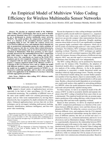
IEEE TRANSACTIONS ON KNOWLEDGE AND DATA ENGINEERING12 @6 . Bitmap d (0,0,0,0) of size four for and bitmap d ç dd ç(0,0,0,0,0) of size 5 for @ are initialized to zeros. Scanning of table 4 will result in (1,1,1,0) and (1,0,0,1,0). Three out of four instances of (i.e., 1, 2, and 3) participate in co-location @6 , so theparticipation ratio for is .75. Similarly, the participation ratio for @ is .4. Therefore, the participation index is min .75, .4 .4.ratios for and@in co-locationAfter the participation indexes are determined, prevalence-based pruning is carried out and non-prevalentco-locations are deleted from the candidate prevalent co-location sets. For each remaining prevalent co-Clocation after prevalence-based pruning, we keep a counter to specify the cardinality of the table instanceCof . All the table instances of the prevalent co-locations in this iteration will be kept for generation ofthe prevalent co-locations of size¿cÀ Aand discarded after the next iteration.Multi-resolution Pruning: Multi-resolution pruning is learned on a summary of spatial data at a coarseresolution using a disjoint partitioning, e.g., pagination imposed by leaves of a spatial index or a grid. Anew neighbor relationship) on partitions is derived from relationshipneighbors if any two instances from each of the two partitions areof a spatial featurecoarse space, wherein each partitionnQ))so that two partitions are)neighbors. We combine all instancesin the partitioning as a new coarse instanceis the number of instances of spatial point featureQ& VQ q n 'in thein cell . For each candidateS EKL M L ¾ U P , we generate its coarse table instance using new coarse instances, new neighbor relationship ) , and its coarse participation index based on the coarse table instance. Multico-location generated byresolution pruning eliminates a co-location if its coarse participation indexes fall below the threshold,because coarse participation never under-estimates the participation index, as shown in section 4.2.We now illustrate multi-resolution pruning by using a simple recti-linear grid for simplicity. In Figure4 a), different shapes represent different point spatial feature types. Every instance has a unique ID in itsspatial feature type and is labeled below it in the figure. Two instances are defined as neighbors if theyare in a commoná ásquare. A grid with uniform cell sizeáis super-imposed on the dataset. Cells

IEEE TRANSACTIONS ON KNOWLEDGE AND DATA ENGINEERINGdCo-location of size 1and coarse level table instancesc1c2c254413103 6798 535263 144a)7(0, 4)(1, 3)(5, 0)(5, 3)1Co-location of size 1and fine level table instances(0, 0) (0, 4)(0, 3) (1, 3)(0, 4) 1(1, 3)(5, 4)12f2f31234567123456789101234111Candidate co-location of size 21Co-location of size 2and fine level table instances30122123Co-location of size 3and fine level table Co-location of size 3and coarse level table instancesc734will be pruned if min preif set to greater than 4/7and algorithm stopsFig. 4.f1(0, 4)(0, 4)(0, 4)(0, 4)(0, 4)(0, 4)(1, 3)(1, 3)(1, 3)(1, 3)(0, 3)(0, 3)(0, 4)(0, 4)(1, 3)(1, 3)(0, 4)(0, 4)(1, 3)(1, 3)(0, 4)(1, 3)(0, 4)(1, 3)(0, 4)(1,3)(0, 4)(1, 3)(0, 4)(1, 3445566Co-location of size 2and coarse level table instancesc4c5c6f6121234344/7 4/4556677889912123434345/10 4/4(0, 4) (0, 3)(0, 4) (0, 4)(0, 4) (1, 3)(1, 3) (0, 3)(1, 3) (0, 4)(1, 3) (1, 3)(5, 3) (5, 4)5/7(0, 4) (0, 4)(0, 4) (1, 3)(1, 3) (0, 4)(1, 3) (1, 3)4/7 4/4(0,3 ) (0, 4)(0, 3) (1, 3)(0, 4) (0, 4)(0, 4) (1, 3)(1, 3) (0, 4)(1, 3) (0, 4)6/10 4/47/10will be pruned if min preif set to 0.6,andwill be further evaluatedand algorithm stopsCandidate co-location of size 3b)Co-location Miner Algorithm with Multi-resolution Pruning Illustration(i,j) refer to cells with an x-axis index of i and a y-axis index of j. In this grid, two cells are coarseneighbors if their centers are in a common square of sizeá á , which imposes an 8-neighborhood (North,South, East, West, North East, North West, South East, South West) on the cells. For example, cell-pairs .i }W 5 .i Z }5 5 . .# }W 5 . T\ }W 5 and .# Z 5 . T\ }W 5 illustrate coarse-neighbors. This coarse-neighborhooddefinition guarantees that two cells are neighbors if there exists a pair of points from each of the two cellswhich are neighbors in the original dataset. The process of multi-resolution pruning is shown as follows.First, we generate coarse table instances of candidate co-locations of size¿;À \by joining the coarsetable instances with the coarse-neighbor relationships.Next, we calculate the participation indexes for all candidate co-locations based on the coarse table " , we add up all the counts of point instances in each coarse instance "with 1s in its corresponding bitmap (E ) and divide this by å instance of å to get the coarse-participation t "qé 5 èY5² Ze Tê since there are 2 coarseratio of feature . For example, in Figure 4 a), coarse EKLY. .xèinstances. For each spatial feature

IEEE TRANSACTIONS ON KNOWLEDGE AND DATA ENGINEERING14 è é , each containing 2 fine-grain instances of è and totally 7 fine-grain instances qé qé 5ë Ze Z \ , yielding coarse participation index E . è [é N5ë of è . Similarly, coarse EKLY. èn 1P . Zm TêeeZe Z 5 4/7. Figure 4 b) shows coarse table instances of co-locations è [ì · è qé and Nìæqé .row instances ofIf the threshold for prevalence is set to 0.6, then co-locationC íandC îcan be pruned by multi-resolutionpruning. We also note that the sizes of coarse table instances are smaller than the sizes of table instancesat fine resolution. This shows the possibility of computation cost saving via multi-resolution pruningfor clustered datasets. Finally, the examples in Figure 4 b) show that the coarse participation ratios andparticipation indexes never underestimate the true participation indexes of the original dataset.D. Generating Co-location RulesThe generate colocation rule function generates all the co-location rules with the user defined conditional probability thresholdïfrom the pre

Data mining approaches can be further divided into a clustering-based map overlay approach and association rule-based approaches. A clustering-based map overlay approach [9], [8] treats every spatial attribute as a map layer and considers spatial clusters (regions) of point-data in each layer as candidates for mining associations. Given * and