Transcription
Alma Mater StudiorumUniversità degli Studi di BolognaFacoltà di Scienze StatisticheCorso di Laurea Magistrale in Sistemi Informativi per l’Azienda e la FinanzaTesi di Laurea in Data Mining e Supporto alle DecisioniComparison of Data MiningTechniques for Insurance ClaimPredictionCandidato:Andrea Dal PozzoloRelatore:Prof. Gianluca MoroCorrelatori:Prof. Gianluca BontempiDott. Yann Aël Le BorgneAnno Accademico 2010/2011 - Sessione II
AbstractThis thesis investigates how data mining algorithms can be used to predictBodily Injury Liability Insurance claim payments based on the characteristicsof the insured customer’s vehicle. The algorithms are tested on real dataprovided by the organizer of the competition. The data present a number ofchallenges such as high dimensionality, heterogeneity and missing variables.The problem is addressed using a combination of regression, dimensionalityreduction, and classification techniques.Questa tesi si propone di esaminare come alcune tecniche di data mining possano essere usate per predirre l’ammontare dei danni che un’assicurazione dovrebbe risarcire alle persone lesionate a partire dalle caratteristiche del veicolo del cliente assicurato. I dati utilizzati sono reali e la loroanalisi presenta diversi ostacoli dati dalle loro grandi dimensioni, dalla loroeterogeneitá e da alcune variabili mancanti. ll problema é stato affrontatoutilizzando una combinazione di tecniche di regressione, di riduzione didimensionalitá e di classificazione.3
4
Contents1 Introduction72 Data Mining algorithms: overview2.1 Data Mining definition and notations . . . . .2.2 Supervised learning . . . . . . . . . . . . . . .2.3 Classification . . . . . . . . . . . . . . . . . .2.3.1 Decision Tree . . . . . . . . . . . . . .2.3.2 Random Forest . . . . . . . . . . . . .2.3.3 Naı̈ve Bayes . . . . . . . . . . . . . . .2.3.4 K-Nearest Neighbors (KNN) . . . . . .2.3.5 Neural Network (NN) . . . . . . . . . .2.3.6 Support Vector Machine (SVM) . . . .2.3.7 Linear discriminant Analysis (LDA) . .2.4 Regression . . . . . . . . . . . . . . . . . . . .2.4.1 Linear model . . . . . . . . . . . . . .2.5 Unsupervised learning . . . . . . . . . . . . .2.5.1 K-means . . . . . . . . . . . . . . . . .2.5.2 Principal Components Analysis (PCA)3 Problem characteristics3.1 Data understanding .3.2 The Gini Index (GI)3.3 Methodology . . . .and. . . . . . .4 Experimental Results4.1 Data preprocessing . .4.2 Regression . . . . . . .4.3 Classification . . . . .4.3.1 Decision Tree .4.3.2 Random Forest.prediction. . . . . . . . . . . . . . . . . . .5.11111315182021222326293031323233strategy. . . . . . . . . . . . . . . . . . . . . . . . . . . . . . . . . . . . . . . . . . . . . . . . . . . . . . .37373940.434343474752.
4.44.54.3.3 Naı̈ve Bayes . . . . . . . . . . . . . . . .4.3.4 K Nearest Neighbors (KNN) . . . . . . .4.3.5 Neural Networks (NN) . . . . . . . . . .4.3.6 Support Vector Machine (SVM) . . . . .4.3.7 Linear Discriminant Analysis (LDA) . .Unsupervised techniques . . . . . . . . . . . . .4.4.1 K-means . . . . . . . . . . . . . . . . . .4.4.2 Principal Components Analysis (PCA) .Submission and final position in the competition.5555576062646467685 Conclusions736 Acknowledgments776
Chapter 1IntroductionWith the increasing power of computer technology, companies and institutions cannowadays store large amounts of data at reduced cost. The amount of available datais increasing exponentially and cheap disk storage makes it easy to store data thatpreviously was thrown away. There is a huge amount of information locked up indatabases that is potentially important but has not yet been explored. The growing sizeand complexity of the databases makes it hard to analyze the data manually, so it isimportant to have automated systems to support the process. Hence there is the needof computational tools able to treat these large amounts of data and extract valuableinformation.In this context, Data Mining provides automated systems capable of processinglarge amounts of data that are already present in databases. Data Mining is used toautomatically extract important patterns and trends from databases seeking regularitiesor patterns that can reveal the structure of the data and answer business problems. DataMining includes learning techniques that fall into the field of Machine learning. Thegrowth of databases in recent years brings data mining at the forefront of new businesstechnologies [WF05].To apply and develop their new research ideas, data scientists need large quantitiesof data. Most of the time however business valuable data is not freely available, soit is not always possible for a data expert to have access to real data. Competitionsare usually the occasion for data miners to access real business data and compete withother people to find the best technique to apply to the data. The Kaggle website(http://www.kaggle.com/) is a web platform where companies have the opportunity topost their data and have it scrutinized by data scientists. In this way data experts havethe opportunity to access real dataset and solve problems with the opportunity to win aprize given by the company.7
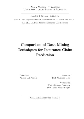
The competition used for this thesis was a Claim Prediction hallenge] proposed by AllstateInsurance. The goal of the competition was to predict the amount of money theinsurance has to pay to its clients. This amount represents an important figure inorder to determine the corresponding premium asked to their customers. Many factorscontribute to the frequency and severity of car accidents including how, where and underwhat conditions people drive, as well as the type of vehicle they use. Bodily InjuryLiability Insurance covers other people’s bodily injury or death for which the insured isresponsible. The company provided data from 2005 to 2007 to contestants, who analyzedcorrelations between vehicle characteristics and bodily injury claims payments to predictclaims payment amounts in 2008. Using the data provided, modelers evaluated howfactors such as horsepower, length and number of cylinders affect the likelihood of aninsured being held responsible for injuring someone in a car accident.Figure 1.1: Claim Prediction competitionThe contribution of this thesis is to analyze and discuss the advantages and disadvantages of the standard techniques used in data mining and machine learning. The thesisfirst presents a general overview of data mining in Chapter 2 and provides a state of the8
art of different learning algorithms. In Chapter 3, we detail the data and the problemaddressed by this competition, and present the methodology that will be used. Chapter4 presents and discusses the experimental results which were obtained. Chapter 5 finallyconcludes the thesis with a summary of the results and the methodology, together withfuture work which could be investigated in order to improve the work presented in thisthesis.9
10
Chapter 2Data Mining algorithms: overview2.1Data Mining definition and notationsData mining is a field of computer science that involves methods from statistics, artificialintelligence, machine learning and data base management. The main goal of data miningis to find hidden patterns in large data sets. This means performing automatic analysisof data in order to find clusters within the data, outliers, association rules and predictionmodels that can explain the data. The information discovered by data mining can belearnt by machine learning algorithms and applied to new data. What is importantis that the patterns found by data mining are useful to explain the data and/or makepredictions from it.Tom Mitchell [Mit97] gives a nice definition of what ‘learning for a computer” means:A computer program is said to learn from experience E with respect to some class oftask T and performance measure P, if its performance at task in T, as measured by P,improves with experience EIn learning program three things must be defined: the task the performance’s measure the source of experience (training experience)Machine learning is the subfield of computer science that deals with the design ofalgorithms and techniques that allow computers to learn [LB09].The goal of Machine Learning is to find algorithms that can learn automatically fromthe past without the need of assistance. The algorithm is trained to learn from data andcome up with a model that can be applied to new data.11
These algorithms are data driven, so they are not guided by the impressions of ahuman expert. To see if an algorithm has effectively learnt something useful or not, itis usually tested with a new data set whose outcome is known in order to evaluate itsoutcome against the real one.Let’s introduce some data mining concepts that will be use in the thesis. Dataset A dataset is a collection of data of the same phenomenon given in atabular form. The columns represent the attributes or variables. The rows, theinstances/examples belonging to the dataset. Each instance has k values, one foreach of the k attributes in the dataset. Attribute / Feature An attribute is one of the available variables present in thedataset. This means that the column of a dataset represent the possible valuestaken by an attribute. Dimension The dimension of a dataset is equivalent to the number of attributespresent in the dataset. In case the dataset is composed of only two variables, itsdimension is two. Training and Testing sets The training and test set are different collection ofdata of the same phenomenon used in supervised learning. The first is used to trainan algorithm to learn, the second to evaluate the learning. Distribution A distribution is a functions that describe the frequencies of thevalues within the phenomenon. Outlier An outlier is an observation that appears to deviate markedly from othermembers of the sample in which it occurs [Gru69].Data mining and Machine learning algorithms can be classified into supervised orunsupervised learning depending on the goal of the algorithm. Supervised methods areused when there is a variable whose value has to be predicted. Such a variable is referredto as response or output variable. In an unsupervised method, the data are not labeledand there is no value to predict or classify.Supervised learning algorithms generate a function that is able to map the input/output values. In these algorithms the data provides examples about the kind of relationshipbetween the input and output variables that has to be learnt. In unsupervised learning,there is no output value, but instead just a collection of input values.Supervised learning algorithms can be further divided into classification and regressionalgorithms. In the case of classification, the goal is to predict qualitative or categorical12
outputs which assume values in a finite set of classes (e.g. True, False or Green , Red,Blue, ecc.) without an explicit order. Categorical variables are also called Factors. Inregression the output to predict is a real-valued number.2.2Supervised learningIn Supervised learning, the training set consists of several input variables and an outputvariable which is a categorical variable in the case of a classification problem and a realvalued number in the case of regression. The goal of supervised algorithms is to uncoverthe relationships between input/output variables and to generalize the function so it canbe applied to new data. The output variables are in general assumed to be dependent onthe inputs. In this thesis input variables will be called X and the output Y .Classification and regression learning algorithms fall into supervised methods becausethey work under the supervision of an output variable. This output variable is called theclass or response value. The success of supervised learning is evaluated by applying themodel on new set of data called test data, for which the values of the output are knownbut not used during the learning stage. The prediction accuracy on this test set can beused as a measure of a model’s ability to predict the response value.A supervised learning therefore requires to have a measure of how well or bad themodel predicts the response variable. This is expressed with a loss function that is usedto assess the adequacy and effectiveness of different methods. Before applying one modelto a test set, the model accuracy is usually estimated using a cross-validation approachwith the training data.The elements of a supervised learning algorithm are: A target operator y(x) that describes the relationship between input-output variables. This is a stochastic process that represents the distribution of y(x) given x,(P (y x)). A training set that contains the data where the relationship between the inputsoutputs variables can be learnt. A prediction model that estimates the input/output variables relationship by meansof a functions and returns a predicted value for each examples. A loss function L(y, ŷ) that is used to measure the goodness of the model by meansof the differences between the predicted output ŷ and the actual output y. A learning procedure that tests different model parameter in order to minimize theloss function and finds the best model for the target function.13
the model space. The learning procedure is an essential part of a learning task, and isthe subject of Section 2.2.2.An overview of the supervised learning setting is given in Figure 2.6.input xTarget functionoutput yTraining seterror L(y, ŷ)Learning procedurePrediction modeloutput ŷFigure 2.1: Supervisedlearning actorsand procedure[LB09].Figure 2.6: The supervisedlearning setting.A trainingset madeof input and outputobservations of the target operator is used by a learning procedure to identify a predictionmodel of the target operator. The goal is to minimize the error between the true output yThe goal ofmodelthe learningprocedureto obtaina modelwhich is able to find theand the predictionŷ, quantifiedby ais lossfunctionL(y, ŷ).dependency between the output and input variable. The model should be general enoughto be 2.3:applieddata anda smallerror. In general,tend toby theExampleLettousnewassumethatreturnthe truerelationshipbetweencomplexx and modelsy is defined2overffit,i.e., theyperformancesto the trainingdata,but andpoorthat astochasticprocessy(x) give x good where N when(0, applied) is a Gaussianrandomnoise,resultsto new data.On thecontraryAsimpletendunderffittrainingset ofwhenN applied100 exampleshas beencollected.linear modelsmodel ofthetoformŷ the1 2 x,data,they cannottherelationship.model. Hencea modelalthoughnotsinceoptimal,could berepresentused as importanta first try informationto representintheTheparameter2space hasis Rto,bethevectorenoughof parametersis performances ( 1 , 2 ). Theleast squarebased ongeneralto return goodin differentdatasetstechnique,without losingthe quadraticloss function,can assessmentbe used as thelearningalgorithmto estimateparametersdiscriminationpower. Theof thegeneralizationabilityis called thevalidation . Thistechniquewillusingbe detailedin Section2.2.3.validation.andthis is donetechniquessuch as cross26A k-fold cross validation consists in partitioning the training data into k smallersubsets of equal size. Then k 1 subsets are used as a training set and the remainingsubset as a test set. This allows to compute the model on a new training set and assessits generalization error on the subset used as the test set. This partition of the trainingset is repeated K times and at each time the subset used for testing is changed. At theend, the validation procedure provides an estimate of the generalization error and thiscan be used to select between different model’s parameters.In the case of a 10 fold cross validation the training data is divided into 10 differentparts of equal size. Then one tenth of the instances present in the training set are usedfor testing and the remaining nine tenth for the training (figure 2.2).Once the first round of validation is completed, another subset of equal size is used fortesting, and the remaining 90% of the instances used for training as before (figure 2.3).The process is iterated 10 times to ensure the all instances become part of the trainingand test set.14
K 10: at each iteration 90% of data are used for training and theremaining 10% for the test.10%10-fold cross-validation90%K 10: at each iteration 90% of data areused for training and theremaining 10% for the test.Figure 2.2: train (blue) and test set (red) used in the first round of a 10 cross validation10%90%Figure 2.3: train (blue) and test set (red) used in the second round of a 10 cross validation2.3ClassificationIn a classification problem the output variable, also called class variable, is a factor takingtwo or more discrete values. The input variables can take either continuous or discretevalues.In the claim prediction competition the problem can be seen as a two-class predictionproblem whereby instances are labeled as positives (P) if the Claim Amount is greaterthen zero and as negatives (N) in the opposite case. Therefore there are four differentcases: an instance is predicted as P and the actual value is also P: this is said to be a true15
positive (TP) an instance is predicted as P but the actual value is N: this is called a false positive(FP) an instance is predicted as N and the actual value is also N: this is a true negative(TN) an instance is predicted as N but the actual value is T: this is a false negative (FN)This information can be summarized into a “Confusion Matrix”, a matrix that makesit easy to visualize how precise the classification is. The columns of the matrix return thenumber of instances in a predicted class, while the rows give the number of instances inthe actual/real class. The number of misclassified instances can be computed summingthe FP and FN instances.Figure 2.4: Confusion MatrixA perfect classifier would have zero FP and zero FN meaning that all the instancesare well classified. The entries of the matrix can also be combined in order to extractother measures. Typical measures obtained by the confusion matrix are: Precision TP / (TP FP) Recall/ Sensitivity TP / P TP / (TP FN) Accuracy (TP TN) / (P N) Specificity TN / (FP TN)These other measures are useful for example when a dataset is unbalanced since theclassifier can be biased towards the class that is more frequent affecting the accuracy.16
For example, in the case where 95% of the instances are positives and only 5% negatives,the classifier could easily classify all the instances as positives leading to an accuracy of95%. For this reason the accuracy is not a reliable measure of classifier’s performance inunbalanced problems [WIK].Another useful tool to assess a binary classifier is the Receiver Operating Characteristic (ROC) Curves. The ROC curve is a plot of the Recall, also called Sensitivity, versus(1 - Specificity), and is obtained by varying the discrimination threshold of the classifier.The ROC curve can also be represented by plotting the fraction of TP out of the positives(true positive rate or TPR) versus the fraction of FP out of the negatives (false positiverate or FPR). For this reason it is also known as a Relative Operating Characteristiccurve, because it is a comparison of two operating characteristics (TPR & FPR) [WIK].In the ROC curve the best possible prediction method would yield a point in the upperleft corner representing no false negative and 100% specificity (no false positive). Onthe contrary a random classification would give a point along a diagonal line (line of nodiscrimination) from the left bottom to the top right corner [WIK]. Different ROC curvesfrom several models can be compared to find optimal models and eliminate suboptimalones.Figure 2.5: ROC curveConfusion matrix and ROC curves do not take into consideration the cost of misclassification and the priori class distribution. The cost of having a high number of falsenegatives may be much higher than the cost of having an equivalent number of falsepositives.17
2.3.1Decision TreeDecision tree algorithms, as the name suggests, are algorithms that can be representedgraphically by a tree with many branches and leaves. Instances are classified going downfrom the root to the leaf nodes [WKRQ 08]. The nodes in the tree are tests for specificattributes. The leaves contain the predictions for the response variable.Trees can be used for both classification and regression problems. In a classificationtree the predicted value is one of the possible levels of the response variable.The Tree construction may be seen as a variable selection method [GE03]; at eachnode the issue is to select the variable to divide upon and how to perform the split.Decision tree algorithms differ in fact from the method of selecting the attribute used totest the instances at each node.The attribute that alone classifies best the data is used at the root, then descendingthe tree the second best attribute is used to split further the data and so on.The term Entropy is used to measure the “impurity” of the training dataset and canbe computed for binary classification problem as well as for classification with the targetattribute taking more levels. If for each node i of a classification tree, the probability ofPthe instance to belong to the k class is pik , the entropy is then calculated aspik log pik .The reduction of entropy can be itself a measure of the information gained partitioningon an attribute [VR02b].Given a tree, to predict a new instances the classification begins at the root and theinstance go down the tree testing different attributes until a leaf is reached. In general adecision tree model works well when: Each attribute of the dataset takes a small number of different levels. Learning rules do not overlap.When the tree algorithm is applied, some common issues are the size of the tree, howto handle missing values/outliers and the appropriate attribute selection at each node.Noise in the data can easily lead to an over fitted tree on the training set giving a modelthat does not perform well in the test set. The size determines the complexity of the treeand has to be neither too simple or too big leading to overfitting.In order to avoid overfitting classical approaches are: Stop growing approaches. Post-pruning approaches.In general, post pruning approaches have been preferred since it may be difficult todetect when to stop the tree growing. Regardless of the method used to avoid overfitting,18
the most important thing is to the determine the correct final size of the tree. There aremany ways to get the correct tree size, including the use of a separate set to determinewhen the further split improves the model and the use of a measure of complexity. Theuse of a separate set to compute the correct size consists in considering each node in thetree as a candidate for pruning. Whenever the tree applied in the test set performs worsethan the original give by the training set, the node is removed and it becomes a leaf.The accuracy of the model applied to the test set increases with the proceeding of pruning.A standard decision tree algorithm for classification problems is the C4.5 decisiontree algorithm that was initially developed by Ross Quinlan [Qui93]. The C4.5 algorithmextends Quinlan’s earlier ID3 tree algorithm to address certain practical issues such asorverfitting and the type of variables accepted in input.Overfitting is a problem that affects all algorithms not only decision trees. It occurswhen there is either noisy data or when the set of training data is not representativeenough because it is too small. In general there is overfitting when there is a model thatis excessively complex and it have poor predicting power when applied to unseen data.With noisy data the ID3 algorithm will create a more complex tree with inconsistencies.C4.5 algorithm is able to use not only binary attribute, but also attributes with manylevels and numerical ones. In the case of numerical attribute, the test is converted to abinary problem by identifying a threshold to see if the instances are greater or smallerthan it. At each node, the criteria to select the attribute is the normalized informationgain (difference in entropy) that results from choosing an attribute for splitting thedata. The attribute with the highest normalized information gain is chosen to make thedecision [WIK].Using the normalized information gain criteria avoids the problem to favor the selection of attributes with many outcomes that happens with the information gain criteria[WKRQ 08]. The growth of the tree terminates when all instances in the training setcan be classified. The class with more number of instances decides the class of the leaf.Pruning the tree is essential to avoid over fitting. The C4.5 algorithm uses a simplification of the cost-complexity pruning use in CART algorithm [DEO11], it is called thereduced error pruning. This method requires a different dataset for prediction. The testset permits evaluation of whether replacing a subtree to a leaf gives an equal or smallernumber of error in the test set. If this is the case the subtree is pruned and replacedby a leaf, with the process of removing branches that do not help continuing until theclassification error starts to increase.19
2.3.2Random ForestRandom forest is an algorithm that consists of many decision trees. It was first developedby Leo Breiman and Adele Cutler [Bre01]. The idea behind it is to build several trees,to have the instance classified by each tree, and to give a “vote” at each class [CZ01].The model uses a “bagging” approach and the random selection of features to build acollection of decision trees with controlled variance. The instance’s class is to the classwith the highest number of votes, the class that occurs the most within the leaf in whichthe instance is placed. In this algorithm, all trees are grown in this way:1. Let N be the number of instances in the training. Sample randomly N instanceswith replacement and use this sample as the training set for growing one tree.2. Let M be the number of input variables. Select a number m smaller than M suchthat at each node, m variables are selected randomly from the M variables, andselect the best split within the m variables. The value of m is held constant duringthe forest growing.3. Each tree is grown unpruned to its largest extent possible.The error of the forest depends on: Trees correlation: the higher the correlation, the higher the forest error rate. The strength of each tree in the forest. A strong tree is a tree with low error. Byusing trees that classify the instances with low error the error rate of the forestdecreases.The correlation and strength of the forest increases with the number m of variablesselected. A smaller m returns a smaller correlation and strength. To improve the prediction’s accuracy, a bootstrap method is used to create different trees. Every time a tree iscreated, one-third of the bootstrap sample is kept aside to estimate the test error. Thesubset that is not included in the tree construction is used as a test set for the same tree.The error of the tree on this test set is called the “out-of-bag” error.This out-of bag (OOB) error is used to get a running unbiased estimate of the classification error as trees are added to the forest and to get estimates of variable importance[CZ01]. Once a tree is built, it is used to predict all data and this allows to computeproximities. Every time two instances fall into the same node, it increases the proximities.This computation is done for each tree and proximities can be used to replace missingvalues. One of the main advantages of this method is it that can handle thousands ofinput variables without variable deletion. On the other hand Random forests do nothandle large numbers of irrelevant features, and are biased in favor of variables with highnumber of levels [WIK].20
2.3.3Naı̈ve BayesThe Naı̈ve Bayes classifier receives the name from the well known Bayes’ theorem [WIK].We first define the Bayes’ theorem before introducing the Naı̈ve Bayes algorithm.Let us suppose that the probability of a certain hypothesis h is P (h), this is also calledthe a priori probability of h. When the probability of an event E is P (E), the conditionalprobability of the event E given that the hypothesis h holds is P (E h). On the contraryP (h E) is the probability that given the event E, h will hold. The Bayes theorem is thendefined by the following equation:P (h E) P (E h)P (h)P (E)In a learning scenario, given that the event E occurred, it is interesting to find whichhypothesis is the most probable in a set of H possible hypotheses. This means to find thehypothesis with the higher P (h E). This probability is also called a posteriori probability.The maximum a posteriori probability hmax is found by:hmax arg max P (h E)hUsing the notion of conditional probability this becomeshmax arg maxhP (E h)P (h)P (E)From this later equation, P (E) can be removed since it is independent of h. Thereforewe get:hmax arg max P (E h)P (h)hIn a classification problem with class variable Y and input variables X, the Bayesoptimal classifier can be defined as the classifier that maximizes the following:arg max P rob(yj x)yjUsing the Bayes theorem this becomes:P (x yi ) P (yi )ŷ arg max P (yi x) PyjP (x
Data Mining algorithms: overview 2.1 Data Mining de nition and notations Data mining is a eld of computer science that involves methods from statistics, arti cial intelligence, machine learning and data base management. The main goal of data mining is to nd hidden patterns in large data sets. This means performing automatic analysis