WIXLIB

ing algorithm. Any particular inductive bias can be helpful or harmful, depending on the problem and the way we approach it. Consider the language modelingtask as an example, where the goal is to estimate a probability distribution oversequences of words. The classical n-gram model makes an independence assumption that each word depends only on the last n 1 words. The assumption helpsto alleviate the problem of data sparsity (Chen and Goodman, 1996) when weperform maximum likelihood estimation. The neural language model (Mikolovet al., 2010) removes this Markov assumption and outperforms the n-gram model.However, this isn’t saying that we cannot add back certain linguistic driven inductive biases that make the model better. These biases might include syntacticstructures (Dyer et al., 2016) or discourse relations (Ji et al., 2016). In this thesis,we specifically look into the question of how to make use of linguistic structuresto form right inductive bias in the neural models, when only limited amounts ofsupervision is available.Neural models are state-of-the-art for many NLP tasks, including speech recognition (Graves et al., 2013), dependency parsing (Kuncoro et al., 2017; Dozat andManning, 2017; Kong et al., 2017) and machine translation (Vaswani et al., 2017).For many applications, the model architecture combines dense representations ofwords (Manning, 2016) with sequential recurrent neural networks (Dyer et al.,2016). Thus, while they generally make use of information about what the wordsare (rather than operating on sequences of characters), they ignore syntactic andsemantic structure or force models to learn it, and thus can be criticized as beingstructurally naive.This thesis argues that explicit structure representations and learned distributedrepresentations can be efficiently combined for improved performance over (i) traditional approaches to structure and (ii) uninformed neural networks that ignoreall but surface sequential structure. As an example, Dyer et al. (2015) yields better2

accuracy than Chen and Manning (2014) by replacing the word representationson the stack with composed representations derived from (partially built) dependency tree structure.In the first part of this thesis, first published as Kong et al. (2015) and Lu et al.(2016), we propose segmental recurrent neural networks (SRNNs) which define,given an input sequence, a joint probability distribution over segmentations of theinput and labelings of the segments. Traditional neural solutions to this problem,e.g., connectionist temporal classification (CTC, Graves et al. (2006a)), reduce thesegmental sequence labeling problem to a sequence labeling problem in the samespirit as BIO tagging. In our model, representations of the input segments (i.e.,contiguous subsequences of the input) are computed by composing their constituent tokens using bi-directional recurrent neural nets, and these segment embeddings are used to define compatibility scores with output labels. Our modelachieves competitive results in phone recognition, handwriting recognition, andjoint word segmentation & POS tagging.In the second part of the thesis, first published as Kong et al. (2017), we propose dynamic recurrent acyclic graphical neural networks (DRAGNN), a modular neural architecture that generalizes the encoder/decoder concept to includeexplicit linguistic structures. The core mechanism of DRAGNN is the TransitionBased Recurrent Unit (TBRU). It represents the linguistic structure a sequence ofdecision/state pairs and guide the building process of the neural networks byfollowing the transitions and encoding the (partial) structures constructed thosetransitions explicitly into the hidden layer activations. We show that our framework is significantly more accurate and efficient than sequence-to-sequence withattention for syntactic dependency parsing and yields more accurate multi-task3

learning for extractive summarization tasks.In the third part of the thesis, we propose to use stochastic attention to modelthe alignment structures explicitly in the neural sequence-to-sequence translationmodel. We regularize the posterior distributions of the latent alignment decisionsusing the posteriors computed from models that make stronger independence assumptions. We show that our posterior regularization scheme leads to substantially improved generalization and several approximations based on importancesampling is either as good as or better than the exact objective in terms of held-outgeneralization.In this thesis, we argue for the importance of explicitly representing structurein neural models. We demonstrate, on three distinct problems, how assumptionsabout structure can be integrated naturally into neural representation learners forNLP problems, without sacrificing computational efficiency. We demonstrate that,when comparing with structurally naive models, models that reason about theinternal linguistic structure of the data demonstrate better generalization performance.4

Chapter 2Notation and RepresentationsIn this thesis, we model the conditional probability in the form of p(y x) usingneural networks, where the goal is to predict the target outputs y from the inputobservations x.We introduce the variable z, where z is the linguistic structure we would liketo explicitly consider. z can take multiple forms. For example, segment structures(chapter 3), parse tree structures (chapter 4), or alignment structures (chapter 5).During the training phrase, when the structure is observable (chapter 4), wecan choose to maximize p(y x) directly. In this setting, the loss is defined asL log p(y, z x)(2.1)If the structure not directly observable from the data, we can treat z as a hiddenvariable, where we follow the marginal likelihood training criterionL log p(y x) log p(y, z x)(2.2)zz can also be given as a soft structure (i.e. , q(z) models probability of z), like inthe case of alignment structure, we can add this to the loss of the model in the5

framework of posterior regularization (Ganchev et al., 2010):L log p(y, z x) γ DKL ( p(z x, y) q(z)),(2.3)zwhere DKL denotes the Kullback–Leibler divergence (Kullback and Leibler, 1951).In the decoding phrase, we are interested in the following prediction problem,y arg max p(y x) arg max p(y, z x).yy(2.4)zWe call this exact decoding (chapter 5). However, summing over all the possible structure z can be expensive or even intractable in many cases. Therefore, wejointly maximize over y and z as a computationally tractable approximation forthe exact decoding method (chapter 3, chapter 4, chapter 5), which is commonlyused in MAP inference problems with latent variables. This is especially convenient when the model can be easily broke down into the following two parts(chapter 4, chapter 5):p(y, z x) p(z x) p(y x, z)(2.5)In some cases (chapter 4, §3.4), given input x, we have a one to many mappingfrom y to z, and a one to one mapping from z to y. In these settings, we use Φ(y)to define the set of all the possible z structures that consistent with y, and φ(z) todefine the corresponding y for z.6

Chapter 3Segmental Recurrent NeuralNetworksIn this chapter, we propose segmental recurrent neural networks (SRNNs)1 whichdefine, given an input sequence, a joint probability distribution over segmentations of the input and labelings of the segments. Representations of the input segments (i.e., contiguous subsequences of the input) are computed by encoding their constituent tokens using bi-directional recurrent neural nets, andthese “segment embeddings” are used to define compatibility scores with output labels. These local compatibility scores are integrated using a global semiMarkov conditional random field (Sarawagi and Cohen, 2004). Both fully supervised training—in which segment boundaries and labels are observed—as wellas partially supervised training—in which segment boundaries are latent—arestraightforward. Applications of fully supervised training include named entity recognition, Chinese word segmentation (Liu et al., 2016) and frame-semanticparsing (Swayamdipta et al., 2017), where boundaries of segments are labeledin the training data. A typical case of partially supervised training is speech1 Firstpublished as Kong et al. (2015) and Lu et al. (2016).7

recognition, where we know the sequence of phonemes during training but theboundaries are not known. Experiments show that, compared to models that donot explicitly represent segments such as BIO tagging schemes and connectionisttemporal classification (CTC, Graves et al. (2006a)), SRNNs obtain substantiallyhigher accuracies.3.1ModelGiven a sequence of input observations x hx1 , x2 , . . . , x x i with length x , a segmental recurrent neural network (SRNN) defines a joint distribution p(y, z x)over a sequence of labeled segments each of which is characterized by a duration (zi Z ) and label (yi Y). The segment durations are constrained such z that i 1 zi x . The length of the output sequence y z is a random variable, and y x with probability 1. We write the starting time of segment i assi 1 j i z j .To motivate our model form, we state several desiderata. First, we are interested in the following prediction problem,y arg max p(y x) arg max p(y, z x) arg max max p(y, z x). (3.1)yyyzzNote the use of joint maximization over y and z as a computationally tractablesubstitute for marginalizing out z; this is commonly done in MAP inference problems with latent variables.Second, for problems where these explicit durations are unavailable at training time, they can be inferred as a latent variable. To train this model, we use amarginal likelihood training criterion,L log p(y x) log p(y, z x).z8(3.2)

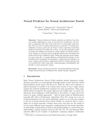
In Eqs. 3.1 and 3.2, the conditional probability of the labeled segment sequence is(assuming kth order dependencies on y): y 1p(y, z x) exp f (yi k:i , zi , x)Z ( x) i 1(3.3)where Z ( x) is an appropriate normalization function. To ensure the expressiveness of f and the computational efficiency of the maximization and marginalization problems in Eqs. 3.1 and 3.2, we use the following definition of f ,f (yi k:i , zi , xsi :si zi 1 ) w φ(V[gy (yi k ); . . . ; gy (yi ); gz (zi ); RNN(csi :si zi 1 ); RNN(csi :si zi 1 )] a) b(3.4) where RNN(csi :si zi 1 ) is a recurrent neural network that computes the forwardsegment embedding by “encoding” the zi -length subsequence of x starting at in dex si ,2 and RNN computes the reverse segment embedding (i.e., traversing thesequence in reverse order), and gy and gz are functions which map the label candidate y and segmentation duration z into a vector representation. The notation[a; b; c] denotes vector concatenation. Finally, the concatenated segment duration,label candidates and segment embedding are passed through a affine transformation layer parameterized by V and a and a nonlinear activation function φ (e.g.,tanh), and a dot product with a vector w and addition by scalar b computes the logpotential for the clique. Our proposed model is equivalent to a semi-Markov conditional random field (Sarawagi and Cohen, 2004) with local features computedusing neural networks. Figure 3.1 shows the model graphically.We chose bi-directional LSTMs (Graves and Schmidhuber, 2005) as the implementation of the RNNs in Eq. 3.4. LSTMs (Hochreiter and Schmidhuber, 1997a)2 Ratherthan directly reading the xi ’s, each token is represented as the concatenation, ci , of aforward and backward over the sequence of raw inputs. This permits tokens to be sensitive tothe contexts, and this is standardly used with neural net sequence labeling models (Graves et al.,2006b).9

are a popular variant of RNNs which have been seen successful in many representation learning problems (Graves and Jaitly, 2014; Karpathy and Fei-Fei, 2015).Bi-directional LSTMs enable effective computation for embeddings in both directions and are known to be good at preserving long distance dependencies, andhence are well-suited for our task.3.2Parameter LearningWe consider two different learning objectives. We use the log loss in our models,other losses such as structured hinge loss can also be used (Tang et al., 2017).Supervised learning In the supervised case, both the segment durations (z) andtheir labels (y) are observed.L log p(y, z x) log Z ( x) log Z ( x, y, z)( x,y,z) D ( x,y,z) DIn this expression, the unnormalized conditional probability of the reference segmentation/labeling, given the input x, is written as Z ( x, y, z).Partially supervised learning In the partially supervised case, only the labelsare observed and the segments (the z) are unobserved and marginalized.L ( x,y) D log p(y x) ( x,y) D z Z ( x,y) ( x,y) D log p(y, z x)log Z ( x) log Z ( x, y)10

Segmentation/Labeling Model(y2y3z1z2z3h 1,3h 4,5h 6,6!h 1,3!h 4,5!h 126Encoder BiRNN(y1Figure 3.1: Graphical model showing a six-frame input and three output segments with durationsz h3, 2, 1i (this particular setting of z is shown only to simplify the layout of this figure; themodel assigns probabilities to all valid settings of z). Circles represent random variables. Shadednodes are observed in training; open nodes are latent random variables; diamonds are deterministic functions of their parents; dashed lines indicate optional statistical dependencies that can beincluded at the cost of increased inference complexity. The graphical notation we use here drawson conventions used to illustrate neural networks and graphical models.For both the fully and partially supervised scenarios, the necessary derivativescan be computed using automatic differentiation or (equivalently) with backwardvariants of the above dynamic programs (Sarawagi and Cohen, 2004).11

3.3Inference with Dynamic ProgrammingWe are interested in three inference problems: (i) finding the most probable segmentation/labeling for a model given a sequence x; (ii) evaluating the partitionfunction Z ( x); and (iii) computing the posterior marginal Z ( x, y), which sumsover all segmentations compatible with a reference sequence y. These can all besolved using dynamic programming. For simplicity, we will assume zeroth orderMarkov dependencies between the yi s. Extensions to the kth order Markov dependencies are straightforward. Since each of these algorithms relies on the forwardand reverse segment embeddings, we first discuss how these can be computedbefore going on to the inference algorithms.3.3.1Computing Segment Embeddings Let h i,j designate the RNN encoding of the input span (i, j), traversing from left to right, and let h i,j designate the reverse direction encoding using RNN. Thereare thus O( x 2 ) vectors that must be computed, each of length O( x ). Naivelythis can be computed in time O( x 3 ), but the following dynamic program reducesthis to O( x 2 ): h i,i h i,j h i,i h i,j RNN( h 0 , ci ) RNN( h i,j 1 , c j ) RNN( h 0 , ci ) RNN( h i 1,j , ci )The algorithm is executed by initializing in the values on the diagonal (representing segments of length 1) and then inductively filling out the rest of the matrix. Inpractice, we often can put a upper bound for the length of a eligible segment thusreducing the complexity of runtime to O( x ). This savings can be substantial for12

very long sequences (e.g., those encountered in speech recognition). We define the concatenation of h i,j and h i,j as the segment embedding of segment i to j. One important advantage of SRNNs over RNNs which simply adoptthe BIO tagging scheme is that we have these explicit representations for arbitrarygiven spans.3.3.2Computing the most probable segmentation/labeling andZ ( x)Figure 3.2: Dynamic programming for the computation of Z ( x). We introduce a auxiliary variableαi basically sum over all the potentials until the point of i in the sequence. By combining thatwith the next segment, (we need to sum over all the y labels there), we get α j . All these partialrepresentations are computed from dynamically constructed neural networks.For the input sequence x, there are 2 x 1 possible segmentations and O( Y x )13

different labelings of these segments, making exhaustive computation of Z ( x) infeasible. Fortunately, the partition function Z ( x) may be computed in polynomialtime with the following dynamic program (Figure 3.2):α0 1αj αi i j y Y exp w φ(V[ gy (y); gz (zi ); RNN(csi :si zi 1 ); RNN(csi :si zi 1 )] a) b .After computing these values, Z ( x) α x . By changing the summations to amax operator (and storing the corresponding arg max values), the maximum aposteriori segmentation/labeling can be computed.Both the partition function evaluation and the search for the MAP outputsrun in time O( x 2 · Y ) with this dynamic program. Adding nth order Markovdependencies between the yi s adds requires additional information in each stateand increases the time and space requirements by a factor of O( Y n ). However,this may be tractable for small Y and n.Avoiding overflow. Since this dynamic program sums over exponentially manysegmentations and labelings, the values in the αi chart can become very large.Thus, to avoid issues with overflow, computations of the αi ’s must be carried outin log space.33.3.3Computing Z ( x, y)To compute the posterior marginal Z ( x, y), it is necessary to sum over all segmentations that are compatible with a label sequence y given an input sequence x.3 Analternative strategy for avoiding overflow in similar dynamic programs is to rescale theforward summations at each timestep (Rabiner, 1989; Graves et al., 2006b). Unfortunately, in asemi-Markov architecture each term in αi sums over different segmentations (e.g., the summationfor α2 will have contain some terms that include α1 and some terms that include only α0 ), whichmeans there are no common factors, making this strategy inapplicable.14

To do so requires only a minor modification of the previous dynamic program totrack how much of the reference label sequence y has been consumed. We introduce the variable m as the index into y for this purpose. The modified recurrencesare:γ0 (0) 1γ j (m) γi (m 1) i j exp w φ(V[ gy (yi ); gz (zi ); RNN(csi :si zi 1 ); RNN(csi :si zi 1 )] a) b .The value Z ( x, y) is γ x

School of Computer Science Carnegie Mellon University 5000 Forbes Ave., Pittsburgh, PA 15213 . to work with the best people in the field — David Weiss, Chris Al-berti, Daniel Andor, Ivan Bogatyy, Hao Zhang, Zhuoran Yu, Kuzman . Thanks my best graduate school friend Ting-Hao (Ken-neth) Huang, for always asking me (benign) questions that I .