WIXLIB

MATHEMATICAL BACKGROUND (CM20219)J. P. CollomosseFigure 1.2: (a) Demonstrating how the dot product can be used to measure the component ofone vector in the direction of another (i.e. a projection, shown here as p). (b) The geometryused to prove a b a b cosθ via the Law of Cosines in equation 1.11.1.3.5Vector NormalisationWe can normalise a vector a by scaling it by the reciprocal of its magnitude:aâ a (1.7)This produces a normalised vector pointing in the same direction as the original (unnormalised) vector, but with unit length (i.e. length of 1). We use the superscript ’hat’notation to indicate that a vector is normalised e.g. â.1.4Vector MultiplicationWe can define multiplication of a pair of vectors in two ways: the dot product (sometimescalled the ‘inner product’, analogous to matrix multiplication), and the cross product(which is sometimes referred to by the unfortunately ambiguous term ‘vector product’).1.4.1Dot ProductThe dot product sums the products of corresponding elements over a pair of vectors. Givenvectors a [a1 , a2 , a3 , a. , an ]T and b [b1 , b2 , b3 , b. , bn ]T , the dot product is defined as:a b a1 b1 a2 b2 a3 b3 . an bnnXai bi (1.8)i 1The dot product is both symmetric and positive definite. It gives us a scalar value that hasthree important uses in Computer Graphics and related fields. First, we can compute thesquare of the magnitude of a vector by taking the dot product of that vector and itself:a a a1 a1 a2 a2 . an annXa2i i 12 a 3(1.9)

MATHEMATICAL BACKGROUND (CM20219)J. P. CollomosseSecond, we can more generally compute a b, the magnitude of one vector a in the directionof another b, i.e. projecting one vector onto another. Figure 1.2a illustrates how a simplerearrangement of equation 1.10 can achieve this.Third, we can use the dot product to compute the angle θ between two vectors (if we normalisethem first). This relationship can be used to define the concept of an angle between vectorsin n dimensional spaces. It is also fundamental to most lighting calculations in Graphics,enabling us to determine the angle of a surface (normal) to a light source.a b a b cosθ(1.10)A proof follows from the “law of cosines”, a general form of Pythagoras’ theorem. Consider is analogous to vectortriangle ABC in Figure 1.2b, with respect to equation 1.10. Side CA analogous to vector b. θ is the angle between CA and CB, and so also vectorsa, and side CBa and b. c 2 a 2 b 2 2 a b cosθc c a a b b 2 a b cos θ(1.11)(1.12)Now consider that c a b (refer back to Figure 1.1):(a b) (a b) a a b b 2 a b cos θa a 2(a b) b b a a b b 2 a b cos θ 2(a b) 2 a b cos θa b a b cos θ(1.13)(1.14)(1.15)(1.16)Another useful result is that we can quickly test for the orthogonality of two vectors bychecking if their dot product is zero.1.4.2Cross ProductTaking the cross product (or “vector product”) of two vectors returns us a vector orthogonal to those two vectors. Given two vectors a [ax , ay , az ]T and B [bx , by , bz ]T , thecross product a b is defined as: ay bz az bya b az bx ax bz (1.17)ax by ay bxThis is often remembered using the mnemonic ‘xyzzy’. In this course we only consider thedefinition of the cross product in 3D. An important Computer Graphics application of thecross product is to determine a vector that is orthogonal to its two inputs. This vector issaid to be normal to those inputs, and is written n in the following relationship (care: notethe normalisation):a b a b sin θn̂A proof is beyond the requirements of this course.4(1.18)

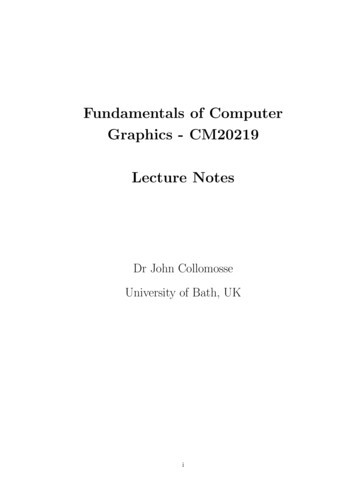
MATHEMATICAL BACKGROUND (CM20219)J. P. CollomosseFigure 1.3: Left: Converting between Cartesian (x, y) and radial-polar (r, θ) form. We treatthe system as a right-angled triangle and apply trigonometry. Right: Cartesian coordinatesare defined with respect to a reference frame. The reference frame is defined by basis vectors(one per axis) that specify how ‘far’ and in what direction the units of each coordinate willtake us.1.5Reference FramesWhen we write down a point in Cartesian coordinates, for example p [3, 2]T , we interpretthat notation as “the point p is 3 units from the origin travelling in the positive direction ofthe x axis, and 2 units from the origin travelling in the positive direction of the y axis”. Wecan write this more generally and succinctly as:p xî y ĵ(1.19)where î [1, 0]T and ĵ [0, 1]T . We call î and ĵ the basis vectors of the Cartesian space,and together they form the basis set of that space. Sometimes we use the term referenceframe to refer to the coordinate space, and we say that the basis set (î, ĵ) therefore definesthe reference frame (Figure 1.3, right).Commonly when working with 2D Cartesian coordinates we work in the reference frame defined by î [1, 0]T , ĵ [0, 1]T . However other choices of basis vector are equally valid, solong as the basis vectors are neither parallel not anti-parallel (do not point in the samedirection). We refer to our ‘standard’ reference frame (î [1, 0]T , ĵ [0, 1]T ) as the rootreference frame, because we define the basis vectors of ‘non-standard’ reference frameswith respect to it.For example a point [2, 3]T defined in reference frame (i [2, 0]T , j [0, 2]T ) would havecoordinates [4, 6]T in our root reference frame. We will return to the matter of convertingbetween reference frames in Chapter 3, as the concept underpins a complete understandingof geometric transformations.5

MATHEMATICAL BACKGROUND (CM20219)1.6J. P. CollomosseCartesian vs. Radial-Polar FormWe have so far recapped on Cartesian coordinate systems. These describe vectors in terms ofdistance along each of the principal axes (e.g. x,y) of the space. This Cartesian form isby far the most common way to represent vector quantities, like the location of points in space.Sometimes it is preferable to define vectors in terms of length, and their orientation. Thisis called radial-polar form (often simply abbreviated to ‘polar form’). In the case of 2Dpoint locations, we describe the point in terms of: (a) its distance from the origin (r), and(b) the angle (θ) between a vertical line (pointing in the positive direction of the y axis), andthe line subtended from the point to the origin (Figure 1.3).To convert from Cartesian form [x, y]T to polar form (r, θ) we consider a right-angled triangleof side x and y (Figure 1.3, left). We can use Pythagoras’ theorem to determine the lengthof hypotenuse r, and some basic trigonometry to reveal that θ tan(y/x) and so:pr x2 y 2(1.20)θ atan(y/x)(1.21)To convert from polar form to Cartesian form we again apply some trigonometry (Figure 1.3,left):1.7x rcosθ(1.22)y rsinθ(1.23)Matrix AlgebraA matrix is a rectangular array of numbers. Both vectors and scalars are degenerate formsof matrices. By convention we say that an (n m) matrix has n rows and m columns; i.e. wewrite (height width). In this subsection we will use two 2 2 matrices for our examples: a11 a12A a21 a22 b11 b12(1.24)B b21 b22Observe that the notation for addressing an individual element of a matrix is xrow,column .1.7.1Matrix AdditionMatrices can be added, if they are of the same size. This is achieved by summing the elementsin one matrix with corresponding elements in the other matrix: a11 a12b11 b12A B a21 a22b21 b22 (a11 b11 ) (a12 b12 ) (1.25)(a21 b21 ) (a22 b22 )This is identical to vector addition.6

MATHEMATICAL BACKGROUND (CM20219)1.7.2J. P. CollomosseMatrix ScalingMatrices can also be scaled by multiplying each element in the matrix by a scale factor.Again, this is identical to vector scaling. sa11 sa12sA (1.26)sa21 sa221.7.3Matrix MultiplicationAs we will see in Chapter 3, matrix multiplication is a cornerstone of many useful geometrictransformations in Computer Graphics. You should ensure that you are familiar with thisoperation. a11 a12b11 b12AB a21 a22b21 b22 (a11 b11 a12 b21 ) (a11 b12 a12 b22 ) (1.27)(a21 b11 a22 b21 ) (a21 b21 a22 b22 )In general each element cij of the matrix C AB, where A is of size (n P ) and B is of size(P m) has the form:cij PXaik bkj(1.28)k 1Not all matrices are compatible for multiplication. In the above system, A must have asmany columns as B has rows. Furthermore, matrix multiplication is non-commutative,which means that BA 6 AB, in general. Given equation 1.27 you might like to write out themultiplication for BA to satisfy yourself of this.Finally, matrix multiplication is associative i.e.:ABC (AB)C A(BC)(1.29)If the matrices being multiplied are of different (but compatible) sizes, then the complexityof evaluating such an expression varies according to the order of multiplication1 .1.7.4Matrix Inverse and the IdentityThe identity matrix I is a special matrix that behaves like the number 1 when multiplyingscalars (i.e. it has no numerical effect):IA A(1.30)The identity matrix has zeroes everywhere except the leading diagonal which is set to 1,e.g. the (2 2) identity matrix is: 1 0(1.31)I 0 11Finding an optimal permutation of multiplication order is a (solved) interesting optimization problem,but falls outside the scope of this course (see Rivest et al. text on Algorithms)7

MATHEMATICAL BACKGROUND (CM20219)J. P. CollomosseThe identity matrix leads us to a definition of the inverse of a matrix, which we writeA 1 . The inverse of a matrix, when pre- or post-multiplied by its original matrix, gives theidentity:AA 1 A 1 A I(1.32)As we will see in Chapter 3, this gives rise to the notion of reversing a geometric transformation. Some geometric transformations (and matrices) cannot be inverted. Specifically, amatrix must be square and have a non-zero determinant in order to be inverted by conventional means.1.7.5Matrix TranspositionMatrix transposition, just like vector transposition, is simply a matter of swapping the rowsand columns of a matrix. As such, every matrix has a transpose. The transpose of A iswritten AT :TA a11 a21a12 a22 (1.33)For some matrices (the orthonormal matrices), the transpose actually gives us the inverseof the matrix. We decide if a matrix is orthonormal by inspecting the vectors that make upthe matrix’s columns, e.g. [a11 , a21 ]T and [a12 , a22 ]T . These are sometimes called columnvectors of the matrix. If the magnitudes of all these vectors are one, and if the vectorsare orthogonal (perpendicular) to each other, then the matrix is orthonormal. Examples oforthonormal matrices are the identity matrix, and the rotation matrix that we will meet inChapter 3.8

Chapter 2Image Representation2.1IntroductionComputer Graphics is principally concerned with the generation of images, with wide rangingapplications from entertainment to scientific visualisation. In this chapter we begin ourexploration of Computer Graphics by introducing the fundamental data structures used torepresent images on modern computers. We describe the various formats for storing andworking with image data, and for representing colour on modern machines.2.2The Digital ImageVirtually all computing devices in use today are digital; data is represented in a discrete formusing patterns of binary digits (bits) that can encode numbers within finite ranges and withlimited precision. By contrast, the images we perceive in our environment are analogue. Theyare formed by complex interactions between light and physical objects, resulting in continuous variations in light wavelength and intensity. Some of this light is reflected in to the retinaof the eye, where cells convert light into nerve impulses that we interpret as a visual stimulus.Suppose we wish to ‘capture’ an image and represent it on a computer e.g. with a scanneror camera (the machine equivalent of an eye). Since we do not have infinite storage (bits),it follows that we must convert that analogue signal into a more limited digital form. Wecall this conversion process sampling. Sampling theory is an important part of ComputerGraphics, underpinning the theory behind both image capture and manipulation — we return to the topic briefly in Chapter 4 (and in detail next semester in CM20220).For now we simply observe that a digital image can not encode arbitrarily fine levels ofdetail, nor arbitrarily wide (we say ‘dynamic’) colour ranges. Rather, we must compromiseon accuracy, by choosing an appropriate method to sample and store (i.e. represent) ourcontinuous image in a digital form.2.2.1Raster Image RepresentationThe Computer Graphics solution to the problem of image representation is to break theimage (picture) up into a regular grid that we call a ‘raster’. Each grid cell is a ‘picture cell’,a term often contracted to pixel. The pixel is the atomic unit of the image; it is coloured uni-9

IMAGE REPRESENTATION (CM20219)J. P. CollomosseFigure 2.1: Rasters are used to represent digital images. Modern displays use a rectangularraster, comprised of W H pixels. The raster illustrated here contains a greyscale image;its contents are represented in memory by a greyscale frame buffer. The values stored in theframe buffer record the intensities of the pixels on a discrete scale (0 black, 255 white).formly — its single colour representing a discrete sample of light e.g. from a captured image.In most implementations, rasters take the form of a rectilinear grid often containing manythousands of pixels (Figure 2.1). The raster provides an orthogonal two-dimensional basiswith which to specify pixel coordinates. By convention, pixels coordinates are zero-indexedand so the origin is located at the top-left of the image. Therefore pixel (W 1, H 1) islocated at the bottom-right corner of a raster of width W pixels and height H pixels. Asa note, some Graphics applications make use of hexagonal pixels instead 1 , however we willnot consider these on the course.The number of pixels in an image is referred to as the image’s resolution. Modern desktopdisplays are capable of visualising images with resolutions around 1024 768 pixels (i.e. amillion pixels or one mega-pixel). Even inexpensive modern cameras and scanners are nowcapable of capturing images at resolutions of several mega-pixels. In general, the greater theresolution, the greater the level of spatial detail an image can represent.2.2.2Hardware Frame BuffersWe represent an image by storing values for the colour of each pixel in a structured way.Since the earliest computer Visual Display Units (VDUs) of the 1960s, it has become common practice to reserve a large, contiguous block of memory specifically to manipulate theimage currently shown on the computer’s display. This piece of memory is referred to as aframe buffer. By reading or writing to this region of memory, we can read or write thecolour values of pixels at particular positions on the display2 .Note that the term ‘frame buffer’ as originally defined, strictly refers to the area of memory reserved for direct manipulation of the currently displayed image. In the early days of1Hexagonal displays are interestingp because all pixels are equidistant, whereas on a rectilinear raster neighbouring pixels on the diagonal are (2) times further apart than neighbours on the horizontal or vertical.2Usually the frame buffer is not located on the same physical chip as the main system memory, but onseparate graphics hardware. The buffer ‘shadows’ (overlaps) a portion of the logical address space of themachine, to enable fast and easy access to the display through the same mechanism that one might access any‘standard’ memory location.10

IMAGE REPRESENTATION (CM20219)J. P. CollomosseGraphics, special hardware was needed to store enough data to represent just that singleimage. However we may now manipulate hundreds of images in memory simultaneously, andthe term ‘frame buffer’ has fallen into informal use to describe any piece of storage thatrepresents an image.There are a number of popular formats (i.e. ways of encoding pixels) within a frame buffer.This is partly because each format has its own advantages, and partly for reasons of backward compatibility with older systems (especially on the PC). Often video hardware can beswitched between different video modes, each of which encodes the frame buffer in a different way. We will describe three common frame buffer formats in the subsequent sections; thegreyscale, pseudo-colour, and true-colour formats. If you do Graphics, Vision or mainstreamWindows GUI programming then you will likely encounter all three in your work at somestage.2.2.3Greyscale Frame BufferArguably the simplest form of frame buffer is the greyscale frame buffer; often mistakenlycalled ‘black and white’ or ‘monochrome’ frame buffers. Greyscale buffers encodes pixelsusing various shades of grey. In common implementations, pixels are encoded as an unsignedinteger using 8 bits (1 byte) and so can represent 28 256 different shades of grey. Usuallyblack is represented by value 0, and white by value 255. A mid-intensity grey pixel has value128. Consequently an image of width W pixels and height H pixels requires W H bytes ofmemory for its frame buffer.The frame buffer is arranged so that the first byte of memory corresponds to the pixel atcoordinates (0, 0). Recall that this is the top-left corner of the image. Addressing thenproceeds in a left-right,

central role in Computer Graphics. Also on this theme, eigenvalue decomposition is dis-cussed and a number of applications relating to visual computing are explored (Chapter 5). 3. OpenGL Programming Discusses how the mathematics on this course can be implemented directly in the C programming language using the OpenGL library (Chapter 4).