WIXLIB

AutoScale: Dynamic, Robust Capacity Management for Multi-Tier Data Center14:3unpredictable changes in request rate, and the full AutoScale policy (see Section 4.3),which builds upon AutoScale-- to handle all forms of changes in load.While AutoScale-- addresses a problem that many others have looked at, it does soin a very different way. Whereas prior approaches aim at predicting the future requestrate and scaling up the number of servers to meet this predicted rate, which is clearlydifficult to do when request rate is, by definition, unpredictable, AutoScale-- does notattempt to predict future request rate. Instead, AutoScale-- demonstrates that it ispossible to achieve SLAs for real-world workloads by simply being conservative in scaling down the number of servers: not turning servers off recklessly. One might thinkthat this same effect could be achieved by leaving a fixed buffer of, say, 20% extraservers on at all times. However, the extra capacity (20% in the above example) shouldchange depending on the current load. AutoScale-- does just this – it maintains justthe right number of servers in the on state at every point in time. This results in muchlower power/resource consumption. In Section 3.5, we evaluate AutoScale-- on a suiteof six different real-world traces, comparing it against five different capacity management policies commonly used in the literature. We demonstrate that in all cases,AutoScale-- significantly outperforms other policies, meeting response time SLAswhile greatly reducing the number of servers needed, as shown in Table III.To fully investigate the applicability of AutoScale--, we experiment with multiplesetup times ranging from 260 seconds all the way down to 20 seconds in Section 3.7and with multiple server idle power consumption values ranging from 140 Watts allthe way down to 0 Watts in Section 3.8. Our results indicate that AutoScale-- canprovide significant benefits across the entire spectrum of setup times and idle power,as shown in Figures 9 and 10.To handle a broader spectrum of possible changes in load, including unpredictablechanges in the request size and server efficiency, we introduce the AutoScale policyin Section 4.3. While prior approaches to dynamic capacity management of multi-tierapplications react only to changes in the request rate, AutoScale uses a novel capacityinference algorithm, which allows it to determine the appropriate capacity regardlessof the source of the change in load. Importantly, AutoScale achieves this without requiring any knowledge of the request rate or the request size or the server efficiency,as shown in Tables V, VI, and VII.To evaluate the effectiveness of AutoScale, we build a three-tier testbed consistingof 38 servers that uses a key-value based workload, involving multiple interleavings ofCPU and I/O within each request. While our implementation involves physically turning servers on and off, one could instead imagine that any idle server that is turnedoff is instead “given away”, and there is a setup time to get the server back. To understand the benefits of AutoScale, we evaluate all policies on three metrics: T95 , the 95thpercentile of response time, which represents our SLA; Pavg , the average power usage;and Navg , the average capacity, or number of servers in use (including those idle andin setup). Our goal is to meet the response time SLA, while keeping Pavg and Navg aslow as possible. The drop in Pavg shows the possible savings in power by turning offservers, while the drop in Navg represents the potential capacity/servers available tobe given away to other applications or to be released back to the cloud so as to save onrental costs.This article makes the following contributions.— We overturn the common wisdom that says that capacity provisioning requires“knowing the future load and planning for it,” which is at the heart of existingpredictive capacity management policies. Such predictions are simply not possiblewhen workloads are unpredictable, and, we furthermore show they are unnecessary, at least for the range of variability in our workloads. We demonstrate thatACM Transactions on Computer Systems, Vol. 30, No. 4, Article 14, Publication date: November 2012.

14:4A. Gandhi et al.Fig. 1. Our experimental testbed.simply provisioning carefully and not turning servers off recklessly achieves better performance than existing policies that are based on predicting current load orover-provisioning to account for possible future load.— We introduce our capacity inference algorithm, which allows us to determine theappropriate capacity at any point of time in response to changes in request rate,request size and/or server efficiency, without any knowledge of these quantities (seeSection 4.3). We demonstrate that AutoScale, via the capacity inference algorithm,is robust to all forms of changes in load, including unpredictable changes in requestsize and unpredictable degradations in server speeds, within the range of our traces.In fact, for our traces, AutoScale is robust to even a 4-fold increase in request size.To the best of our knowledge, AutoScale is the first policy to exhibit these formsof robustness for multi-tier applications. As shown in Tables V, VI, and VII, otherpolicies are simply not comparable on this front.2. EXPERIMENTAL SETUP2.1. Our Experimental TestbedFigure 1 illustrates our data center testbed, consisting of 38 Intel Xeon servers, eachequipped with two quad-core 2.26 GHz processors. We employ one of these servers asthe front-end load generator running httperf [Mosberger and Jin 1998] and anotherserver as the front-end load balancer running Apache, which distributes requests fromthe load generator to the application servers. We modify Apache on the load balancerto also act as the capacity manager, which is responsible for turning servers on andoff. Another server is used to store the entire data set, a billion key-value pairs, on adatabase.Seven servers are used as memcached servers, each with 4GB of memory forcaching. The remaining 28 servers are employed as application servers, which parsethe incoming php requests and collect the required data from the back-end memcachedservers. Our ratio of application servers to memcached servers is consistent with thetypical ratio of 5:1 [Facebook 2011].We employ capacity management on the stateless application servers only, as theymaintain no volatile state. Stateless servers are common among today’s applicationplatforms, such as those used by Facebook [Facebook 2011], Amazon [DeCandia et al.2007] and Windows Live Messenger [Chen et al. 2008]. We use the SNMP communication protocol to remotely turn application servers on and off via the power distributionunit (PDU). We monitor the power consumption of individual servers by reading theACM Transactions on Computer Systems, Vol. 30, No. 4, Article 14, Publication date: November 2012.

AutoScale: Dynamic, Robust Capacity Management for Multi-Tier Data Center14:5power values off of the PDU. The idle power consumption for our servers is about 140W(with C-states enabled) and the average power consumption for our servers when theyare busy or in setup is about 200W.In our experiments, we observed the setup time for the servers to be about 260seconds. However, we also examine the effects of lower setup times that could either bea result of using sleep states (which are prevalent in laptops and desktop machines, butare not well supported for server architectures yet), or using virtualization to quicklybring up virtual machines. We replicate this effect by not routing requests to a serverif it is marked for sleep, and by replacing its power consumption values with 0W. Whenthe server is marked for setup, we wait for the setup time before sending requests tothe server, and replace its power consumption values during the setup time with 200W.2.2. WorkloadWe design a key-value workload to model realistic multi-tier applications such as thesocial networking site, Facebook, or e-commerce companies like Amazon [DeCandiaet al. 2007]. Each generated request (or job) is a php script that runs on the application server. A request begins when the application server requests a value for a keyfrom the memcached servers. The memcached servers provide the value, which itselfis a collection of new keys. The application server then again requests values for thesenew keys from the memcached servers. This process can continue iteratively. In ourexperiments, we set the number of iterations to correspond to an average of roughly3,000 key requests per job, which translates to a mean request size of approximately120 ms, assuming no resource contention. The request size distribution is highly variable, with the largest request being roughly 20 times the size of the smallest request.We can also vary the distribution of key requests by the application server. In thispaper we use the Zipf [Newman 2005] distribution, whereby the probability of generating a particular key varies inversely as a power of that key. To minimize the effects ofcache misses in the memcached layer (which could result in an unpredictable fractionof the requests violating the T95 SLA), we tune the parameters of the Zipf distributionso that only a negligible fraction of requests miss in the memcached layer.2.3. Trace-Based ArrivalsWe use a variety of arrival traces to generate the request rate of jobs in our experiments, most of which are drawn from real-world traces. Table I describes these traces.In our experiments, the seven memcached servers can together handle at most 800 jobrequests per second, which corresponds to roughly 300,000 key requests per secondat each memcached server. Thus, we scale the arrival traces such that the maximumrequest rate into the system is 800 req/s. Further, we scale the duration of the tracesto 2 hours. We evaluate our policies against the full set of traces (see Table III forresults).3. RESULTS: CHANGING REQUEST RATESThis section and the next both involve implementation and performance evaluation ofa range of capacity management policies. Each policy will be evaluated against thesix traces described in Table I. We will present detailed results for the Dual phasetrace and show summary results for all traces in Table III. The Dual phase trace ischosen because it is quite bursty and also represents the diurnal nature of typical datacenter traffic, whereby the request rate is low for a part of the day (usually the nighttime) and is high for the rest (day time). The goal throughout will be to meet 95%ileACM Transactions on Computer Systems, Vol. 30, No. 4, Article 14, Publication date: November 2012.

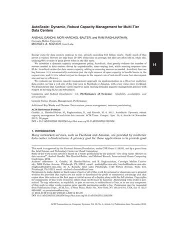
14:6A. Gandhi et al.Table I. Description of the Traces We Use for Experimentsguarantees of T95 400 500 ms1 , while minimizing the average power consumed bythe application servers, Pavg , or the average number of application servers used, Navg .Note that Pavg largely scales with Navg .For capacity management, we want to choose the number of servers at time t, k(t),such that we meet a 95 percentile response time goal of 400 500 ms. Figure 2 showsmeasured 95 percentile response time at a single server versus request rate. Accordingto this figure, for example, to meet a 95 percentile goal of 400 ms, we require therequest rate to a single server to be no more than r 60 req/s. Hence, if the totalrequest rate into the data center at some time t is say, R(t) 300 req/s, we know thatwe need at least k 300/r 5 servers to ensure our 95 percentile SLA.3.1. AlwaysOnThe AlwaysOn policy [Chen et al. 2008; Horvath and Skadron 2008; Verma et al. 2009]is important because this is what is currently deployed by most of the industry. The1 It would be equally easy to use 90%ile guarantees or 99%ile guarantees. Likewise, we could easily haveaimed for 300ms or 1 second response times rather than 500ms. Our choice of SLA is motivated by recentstudies [DeCandia et al. 2007; Krioukov et al. 2010; Meisner et al. 2011; Urgaonkar and Chandra 2005] thatindicate that 95 percentile guarantees of hundreds of milliseconds are typical.ACM Transactions on Computer Systems, Vol. 30, No. 4, Article 14, Publication date: November 2012.

AutoScale: Dynamic, Robust Capacity Management for Multi-Tier Data CenterFig. 2. A single server can optimally handle 60 req/s.14:7Fig. 3. AlwaysOn.policy selects a fixed number of servers, k, to handle the peak request rate and alwaysleaves those servers on. In our case, to meet the 95 percentile SLA of 400ms, we setk R peak /60 , where R peak 800 req/s denotes the peak request rate into the system.Thus, k is fixed at 800/60 14.Realistically, one doesn’t know R peak , and it is common to overestimate R peak by afactor of 2 (see, e.g., [Krioukov et al. 2010]). In this article, we empower AlwaysOn, byassuming that R peak is known in advance.Figure 3 shows the performance of AlwaysOn. The solid line shows kideal , the idealnumber of servers/capacity which should be on at any given time, as given by k(t) R(t)/60 . Circles are used to show kb usy idle , the number of servers which are actuallyon, and crosses show kb usy idle setup , the actual number of servers that are on or in setup.For AlwaysOn, the circles and crosses lie on top of each other since servers are never 14 for AlwaysOn, while Pavg 2323W, within setup. Observe that Navg 80060similar values for the different traces in Table III.3.2. ReactiveThe Reactive policy (see, e.g., Urgaonkar and Chandra [2005]) reacts to the currentrequest rate, attempting to keep exactly R(t)/60 servers on at time t, in accordancewith the solid line. However, because of the setup time of 260s, Reactive lags in turningservers on. In our implementation of Reactive, we sample the request rate every 20seconds, adjusting the number of servers as needed.Figure 4(a) shows the performance of Reactive. By reacting to current request rateand adjusting the capacity accordingly, Reactive is able to bring down Pavg and Navgby as much as a factor of two or more, when compared with AlwaysOn. This is a hugewin. Unfortunately, the response time SLA is almost never met and is typically exceeded by a factor of at least 10–20 (as in Figure 4(a)), or even by a factor of 100 (seeTable III).3.3. Reactive with Extra CapacityOne might think the response times under Reactive would improve a lot by just addingsome x% extra capacity at all times. This x% extra capacity can be achieved by runningReactive with a different r setting. Unfortunately, for this trace, it turns out that tobring T95 down to our desired SLA, we need 100% extra capacity at all times, whichcorresponds to setting r 30. This brings T95 down to 487 ms, but causes power to jumpup to the levels of AlwaysOn, as illustrated in Figure 4(b). It is even more problematicthat each of our six traces in Table I requires a different x% extra capacity to achieveACM Transactions on Computer Systems, Vol. 30, No. 4, Article 14, Publication date: November 2012.

14:8A. Gandhi et al.Fig. 4. (a) Reactive and (b) Reactive with extra capacity.the desired SLA (with x% typically ranging from 50% to 200%), rendering such a policyimpractical.3.4. PredictivePredictive policies attempt to predict the request rate 260 seconds from now. Thissection describes two policies that were used in many papers [Bodı́k et al. 2009;Grunwald et al. 2000; Pering et al. 1998; Verma et al. 2009] and were found to be themost powerful by Krioukov et al. [2010].Predictive - Moving Window Average (MWA). In the MWA policy, we consider a“window” of some duration (say, 10 seconds). We average the request rates during thatwindow to deduce the predicted rate during the 11th second. Then, we slide the windowto include seconds 2 through 11, and average those values to deduce the predicted rateduring the 12th second. We continue this process of sliding the window rightward untilwe have predicted the request rate at time 270 seconds, based on the initial 10 secondswindow.If the estimated request rate at second 270 exceeds the current request rate, wedetermine the number of additional servers needed to meet the SLA (via the k R/r formula) and turn these on at time 11, so that they will be ready to run at time 270.If the estimated request rate at second 270 is lower than the current request rate, welook at the maximum request rate, M, during the interval from time 11 to time 270.If M is lower than the current request rate, then we turn off as many servers as wecan while meeting the SLA for request rate M. Of course, the window size affects theperformance of MWA. We empower MWA by using the best window size for each trace.Figure 5(a) shows that the performance of Predictive MWA is very similar to whatwe saw for Reactive: low Pavg and Navg values, beating AlwaysOn by a factor of 2, buthigh T95 values, typically exceeding the SLA by a factor of 10 to 20.Predictive - Linear Regression (LR). The LR policy is identical to MWA except that,to estimate the request rate at time 270 seconds, we use linear regression to match thebest linear fit to the values in the window. Then we extend our line out by 260 secondsto get a prediction of the request rate at time 270 seconds.The performance of Predictive LR is worse than that of Predictive MWA. Responsetimes are still bad, but now capacity and power consumption can be bad as well. Theproblem, as illustrated in Figure 5(b), is that the linear slope fit used in LR can end upovershooting the required capacity greatly.ACM Transactions on Computer Systems, Vol. 30, No. 4, Article 14, Publication date: November 2012.

AutoScale: Dynamic, Robust Capacity Management for Multi-Tier Data Center14:9Fig. 5. (a) Predictive: MWA and (b) Predictive: LR.Table II. The (In)sensitivity of AutoScale--’s Performance to twaithhhhhhTracetwaithhhhhDual phase[nlanr 7W7.2445ms1,490W8.83.5. AutoScale One might think that the poor performance of the dynamic capacity management policies we have seen so far stems from the fact that they are too slow to turn servers onwhen needed. However, an equally big concern is the fact that these policies are quickto turn servers off when not needed, and hence do not have those servers availablewhen load subsequently rises. This rashness is particularly problematic in the case ofbursty workloads, such as those in Table I.AutoScale-- addresses the problem of scaling down capacity by being very conservative in turning servers off while doing nothing new with respect to turning serverson (the turning on algorithm is the same as in Reactive). We will show that by simplytaking more care in turning servers off, AutoScale-- is able to outperform all the priordynamic capacity management policies we have seen with respect to meetings SLAs,while simultaneously keeping Pavg and Navg low.When to Turn a Server Off? Under AutoScale--, each server decides autonomouslywhen to turn off. When a server goes idle, rather than turning off immediately, itsets a timer of duration twait and sits in the idle state for twait seconds. If a requestarrives at the server during these twait seconds, then the server goes back to the busystate (with zero setup cost); otherwise, the server is turned off. In our experiments forAutoScale--, we use a twait value of 120s. Table II shows that AutoScale-- is largelyinsensitive to twait in the range twait 60s to twait 260s. There is a slight increase inPavg (and Navg ) and a slight decrease in T95 when twait increases, due to idle serversstaying on longer.The idea of setting a timer before turning off an idle server has been proposed before(see, e.g., Kim and Rosing [2006], Lu et al. [2000], and Iyer and Druschel [2001]), however, only for a single server. For a multi-server system, independently setting timersfor each server can be inefficient, since we can end up with too many idle servers. Thus,we need a more coordinated approach for using timers in our multiserver system thattakes routing into account, as explained here.ACM Transactions on Computer Systems, Vol. 30, No. 4, Article 14, Publication date: November 2012.

14:10Fig. 6. For a single server, packing factor, p 10.A. Gandhi et al.Fig. 7. AutoScale--.How to Route Jobs to Servers?. Timers prevent the mistake of turning off a serverjust as a new arrival comes in. However, they can also waste power and capacity byleaving too many servers in the idle state. We’d basically like to keep only a smallnumber of servers (just the right number) in this idle state.To do this, we introduce a routing scheme that tends to concentrate jobs onto a smallnumber of servers, so that the remaining (unneeded) servers will naturally “time out.”Our routing scheme uses an index-packing idea, whereby all on servers are indexedfrom 1 to n. Then, we send each request to the lowest numbered on server that currently has fewer than p requests, where p stands for packing factor and denotes themaximum number of requests that a server can serve concurrently and meet its response time SLA. For example, in Figure 6, we see that to meet a 95%ile guaranteeof 400 ms, the packing factor is p 10 (in general, the value of p depends on thesystem in consideration). When all on servers are already packed with p requestseach, additional request arrivals are routed to servers via the join-the-shortest-queuerouting.In comparison with all the other policies, AutoScale-- hits the “sweet spot” of lowT95 as well as low Pavg and Navg . As seen from Table III, AutoScale-- is close tothe response time SLA in all traces except for the Big spike trace. Simultaneously,the mean power usage and capacity under AutoScale-- is typically significantly betterthan AlwaysOn, saving as much as a factor of two in power and capacity.Figure 7 illustrates how AutoScale-- is able to achieve these performance results.Observe that the crosses and circles in AutoScale-- form flat constant lines, insteadof bouncing up and down, erratically, as in the earli

the servers in a multi-tier data center are application servers, which are stateless, and are thus easy to turn off or give away-for example, one reported ratio of application servers to data servers is 5:1 [Facebook 2011]. We therefore focus our attention on dynamic capacity management of these front-end application servers.