Transcription
The FeedbackLoop7.1 n INTRODUCTIONNow that we are prepared with a good understanding of process dynamics, wecan begin to address the technology for automatic process control. The goals ofprocess control—safety, environmental protection, equipment protection, smoothoperation, quality control, and profit—are achieved by maintaining selected plantvariables as close as possible to their best conditions. The variability of variablesabout their best values can be reduced by adjusting selected input variables usingfeedback control principles. As explained in Chapter 1, feedback makes use ofan output of a system in deciding the way to influence an input to the system,and the technology presented in this part of the book explains how to employfeedback. This chapter builds on the chapters in Part I of the book, which weremore qualitative and descriptive, by establishing the key quantitative aspects of acontrol system.It is important to emphasize that we are dealing with the control system, whichinvolves the process and instrumentation as well as the control calculations. Thus,this chapter begins with a section on the feedback loop in which all elements arediscussed. Then, reasons for control are reviewed, and because engineers shouldalways be prepared to define measures of the effectiveness of their efforts, quantitative measures of control performance are defined for key disturbances; thesemeasures are used throughout the remainder of the book. Because the processusually has several input and output variables, initial criteria are given for selecting the variables for a control loop. Finally, several general approaches to feedback
212control, ranging from manual to automated methods, are discussed, along withguidelines for when to employ each approach.CHAPTER 7The Feedback Loop7.2 Q PROCESS AND INSTRUMENT ELEMENTSOF THE FEEDBACK LOOPAll elements of the feedback loop can affect control performance. In this section,the process and instrument elements of a typical loop, excluding the control calculation, are introduced, and some quantitative information on their dynamics isgiven. This analysis provides a means for determining which elements of the loopintroduce significant dynamics and when the dynamics of some fast elements canusually be considered negligible.A typical feedback control loop is shown in Figure 7.1. This discussion willaddress each element of the loop, beginning with the signal that is sent to theprocess equipment. This signal could be determined using feedback principlesby a person or automatically by a computing device. Some key features of eachelement in the control loop are summarized in Table 7.1.The feedback signal in Figure 7.1 has a range usually expressed as 0 to 100%,whether determined by a controller or set manually by a person. When the signal istransmitted electronically, it usually is converted to a range of 4 to 20 milliamperes(mA) and can be transmitted long distances, certainly over one mile. When thesignal is transmitted peumatically, it has a range of 3 to 15 psig and can only betransmitted over a shorter distance, usually limited to about 400 meters unlessspecial signal reinforcement is provided. Pneumatic transmission would normallybe used only when the controller is performing its calculations pneumatically,which is not common with modern equipment. Naturally, the electronic signalFeedbackDisplay200-300'C0-100%- — 4-20mA4-20mACompressedair3-15 psiValveThermocouplein thermowellProcessFIGURE 7.1Process and instrument elements in a typical control loop.
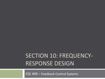
TABLE 7.1213Key features of control loop elements, excluding the processLoop element*Functiontypical rangeController outputInitiate signal at aremote locationintended for the finalelementCarry signal fromcontroller to finalelement and from thesensor to the controllerChange transmissionsignal to onecompatible with finalelementImplement desiredchange in processMeasure controlledvariableOperator/controller use0-100%TransmissionSignal conversionFinal control elementSensorTypical dynamicresponse, t63% Process andInstrument Elementsof the Feedback LoopPneumatic: 3-15 psig Pneumatic: 1-5 sElectronic: 4-20milliamp (mA)Electronic to pneumatic:4-20 mA to 3-15 psigSensor to electronic:mV to 4-20 mAValve: 0-100% openElectronic:Instantaneous0.5-1.0 sScale selected to givegood accuracy, e.g.,200-300 CTypically from a fewseconds to severalminutes1-4 sThe terms input and output are with respect to a controller.**Time for output to reach 63% after step input.S«»KSK!sFiWSsSSC transmission is essentially instantaneous; the pneumatic signal requires severalseconds for transmission. Note that the standard signal ranges (e.g., 4 to 20 mA)are very important so that equipment manufactured by different suppliers can beinterchanged.At the process unit, the output signal is used to adjust the final control element:the equipment that is manipulated by the control system. The final control elementin the example, as in over 90 percent of process control applications, is a valve. Thevalve percent opening could be set by an electrical motor, but this is not usuallydone because of the danger of explosion with the high-amperage power supply amotor would require. The alternative power supply typically used is compressed air.The signal is converted from electrical to pneumatic; 3 to 15 psig is the standardrange of the pneumatic signal. The conversion is relatively accurate and rapid,as indicated by the entry for this element in Table 7.1. The pneumatic signal istransmitted a short distance to the control valve, which is specially designed toadjust its percent opening based on the pneumatic signal. Control valves respondrelatively quickly, with typical time constants ranging from 1 to 4 sec.The general principles of a control valve are demonstrated in Figure 7.2.The process fluid flows through the opening in the valve, with the amount open(or resistance to flow) determined by the valve stem position. The valve stemAir pressureDiaphragmValve plug and seatFIGURE 7.2Schematic of control valve.
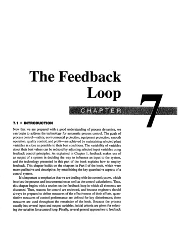
2 1 4 i s c o n n e c t e d t o t h e d i a p h r a g m , w h i c h i s a fl e x i b l e m e t a l s h e e t t h a t c a n b e n d i nHMfe MWBiiiM kaMiii response to forces. The two forces acting on the diaphragm are the spring andchapter 7 the variable pressure from the control signal. For a zero control signal (3 psig),The Feedback Loop the diaphragm in Figure 7.2 would be deformed upward because of the greaterforce from the spring, and the valve stem would be raised, resulting in the greatestopening for flow. For a maximum signal (15 psig), the diaphragm in Figure 7.2would be deformed downward by the greater force from the air pressure, andthe stem would be lowered, resulting in the minimum opening for flow. Otherarrangements are possible, and selection criteria are presented in Chapter 12.After the final control element has been adjusted, the process responds to thechange. The process dynamics vary greatly for the wide range of equipment in theprocess industries, with typical dead times and time constants ranging from a fewseconds (or faster) to hours. When the process is by far the slowest element in thecontrol loop, the dynamics of the other elements are negligible. This situation iscommon, but important exceptions occur, as demonstrated in Example 7.1.The sensor responds to the change in plant conditions, preferably indicatingthe value of a single process variable, unaffected by all other variables. Usually,the sensor is not in direct contact with the potentially corrosive process materials; therefore, the protective equipment or sample system must be included in thedynamic response. For example, a thin thermocouple wire responds quickly to achange in temperature, but the metal sleeve around the thermocouple, the thermowell, can have a time constant of 5 to 20 sec. Most sensor systems for flow,pressure, and level have time constants of a few seconds. Analyzers that performcomplex physicochemical analyses can have much slower responses, on the orderof 5 to 30 minutes or longer; they may be discrete, meaning that a new analyzerresult becomes available periodically, with no new information between results.Physical principles and performance of sensors are diverse, and the reader is encouraged to refer to information in the additional resources from Chapter 1 onsensors for further details.The sensor signal is transmitted to the controller, which we are considering tobe located in a remote control room. The transmission could be pneumatic (3 to15 psig) or electrical (4 to 20 mA). The controller receives the signal and performsits control calculation. The controller can be an analog system; for example, anelectronic analog controller consists of an electrical circuit that obeys the sameequations as the desired control calculations (Hougen, 1972). For the next fewchapters, we assume that the controller is a continuous electronic controller thatperforms its calculations instantaneously, and we will see in Chapter 11 that essentially the same results can be obtained by a very fast digital computer, as isused in most modern control equipment.EXAMPLE 7.1.The dynamic responses of two process and instrumentation systems similar to Figure 7.1, without the controller, are evaluated in this exercise. The system involveselectronic transmission, a pneumatic valve, a first-order-with-dead-time process,and a thermocouple in a thermowell. The dynamics of the individual elements aregiven in Table 7.2 with the time in seconds for two different systems, A and B. Thedynamics of the entire loop are to be determined. The question could be stated,"How does a unit step change in the manual output affect the displayed variable,
TABLE 7.2215Dynamic models for elements in Example 7.1Process andInstrument Elementsof the Feedback LoopElementUnits*Case ACase BManual stationTransmissionmA/% output0.161.00.161.0Signal conversionFinal elementProcessSensorpsi/mA%open/psi C/psimV/ CmA/mV0.75/(0.5* 1)8.33/(1.5* 1)1.84e-107(3* l)0.11/(10*4-1)1.48/(0.51*4-1)1.00.75/(0.5* 1.48/(0.51*4-1)1.0 C/mA6.25/(1.0*4-1)6.25/(1.0*4-1)Signal conversionTransmissionDisplay*Time is in seconds.l*j8W!»ISflIBtJKKMHBI which is also the variable available for control, in the control house?" Note that thetwo systems are identical except for the process transfer functions.The physical system in this problem and shown in Figure 7.1 is recognizedas a series of noninteracting systems. Therefore, equation (5.40) can be appliedto determine the transfer function of the overall noninteracting series system. Theresult for Case B isYjs)Xis)n-\ f]G„ ,(*)1 0-100sYjs) 5)gXis) (0.5* 4- 1)(1.55 4- 0(300* 4- 0(10* 4- 0(0.51* 4- 0(* 4- 0Before the simulation results are presented for this example, it is worthwhileperforming an approximate analysis, using the simple approximation introducedin Chapter 5 for series processes. The overall gains and approximate 63 percenttimes for both systems that relate the manual signal to the display are shown inthe following table:Case A Case BProcess gain KP Y\ K,Time to 63% E(r;4-0()1.84 1.84% 17.5 % 413.5'C/(% controller output)seconds2000FIGURE 7.3The two cases have been simulated, and the results are plotted in Figure 7.3a ando. The results of the approximate analysis compare favorably with the simulations.Note that for system A, which involves a fast process, the sensor and final elementcontribute significant dynamics, resulting in a substantial difference between thetrue process temperature and the displayed value of the temperature, which wouldbe used for feedback control. In system B the process dynamics are much slower,Transient response for Example 7.1 witha 1% step input change at time 0.(a) Case A; ib) Case B.
216CHAPTER 7The Feedback Loopand the dynamic effects of all other elements in the loop are negligible. This is adirect consequence of the time-domain solution to the model of this process for astep (1/*) input, which has the formY\t) C, 4- C2e t/T* C3e-"« Clearly, a slow "mode" due to one especially long time constant will dominatethe dynamic response, with the faster elements essentially at quasi-steady state.One would expect that a dynamic analysis that considered the process alonefor control design would not be adequate for Case A but would be adequate forCase B.HWWW#%8gIt is worth recalling that the empirical methods for determining the "process"dynamics presented in Chapter 6 involve changes to the manipulated signal andmonitoring the response of the sensor signal as reported to the control system. Thus,the resulting model includes all elements in the loop, including instrumentation andtransmission. Since the experiments usually employ the same instrumentation usedsubsequently for implementing the control system, the dynamic model identifiedis between the controller output and input—in other words, the system "seen" bythe controller. This seems like the appropriate model for use in design controlsystems, and that intuition will be supported by later analysis.7.3 eh SELECTING CONTROLLED AND MANIPULATEDVA R I A B L E SFeedback control provides a connection between the controlled and manipulatedvariables. Perhaps the most important decision in designing a feedback control system involves the selection of variables for measurement and manipulation. Someinitial criteria are introduced in this section and applied to the continuous-flowchemical reactor in Figure 7.4. As more details of feedback control are presented,further criteria will be presented throughout Part III for a single-loop controller.We begin by considering the controlled variable, which is selected so that thefeedback control system can achieve an important control objective. The sevencategories of control objectives were introduced in Chapter 2 and are repeatedbelow.Control objectiveFIGURE 7.4Continuous-flow chemical reactorexample for selecting control loopvariables.1. Safety2. Environmental protection3. Equipment protection4. Smooth plant operationand production rate5. Product quality — -6. Profit optimization7. Monitoring and diagnosisProcess variableSensorConcentration of — reactant A in the effluentAnalyzer in reactoreffluent measuringthe mole % A
From none to several controlled variables may be associated with each control 217objective. Here, we consider the product quality objective and decide that the most laiiiftiMiiiimportant process variable associated with product quality is the concentration of Selecting Controlledreactant A in the reactor effluent. The process variable must be measured in real and Manipulatedtime to make it available to the computer, and the natural selection for the sensor Variableswould be an analyzer in the effluent stream. In practice, an onstream analyzermight not exist or might be too costly; for the next few chapters we will assumethat a sensor is available to measure the key process variable and defer discussionsof using substitute (inferential) variables, which are more easily measured, untillater chapters.The second key decision is the selection of the manipulated variable, becausewe must adjust some process variable to affect the process. First, we identifyall input variables that influence the measured variable. The input variables aresummarized below for the reactor in Figure 7.4.Input variables that affect Selected adjustable flow Manipulated valvethe measured variableDisturbances:Feed temperatureSolvent flow rateFeed composition, before mixCoolant inlet temperatureAdjustable:F l o w o f p u r e A F l o w o f p u r e A v AFlow of coolantSix important input variables are identified and separated into two categories:those that cannot be adjusted (disturbances) and those that can be adjusted. Ingeneral, the disturbance variables change due to changes in other plant units andin the environment outside the plant, and the control system should compensatefor these disturbances. Disturbances cannot be used as manipulated variables.Only adjustable variables can be candidates for selection as a manipulatedvariable. To be an adjustable flow, a valve must influence the flow. (In general,manipulated variables include adjustable motor speeds and heater power, and soforth, but for the current discussion, we restrict the discussion to valves.) Criteriafor selecting an adjustable variable include1. Causal relationship between the valve and controlled variable (required)2. Automated valve to influence the selected flow (required)3. Fast speed of response (desired)4. Ability to compensate for large disturbances (desired)5. Ability to adjust the manipulated variable rapidly and with little upset to theremainder of the plant (desired)As a method for ensuring that the manipulated variable has a causal relationshipon the controlled variable, the dynamic model between the valve and controlled
218variable must have a nonzero value, i.e., ACa/AFA Kp 0. An importantaspect of chemical plant design involves providing streams which accommodatethe five criteria above; examples are cooling water, steam, and fuel gas, which aredistributed and made available throughout a plant.Two potential adjustable flows exist in this example, and based on the information available, either is acceptable. For the present, we will arbitrarily selectthe valve affecting the flow of pure component A, uA. After we have analyzed theeffects of feedback dynamics more thoroughly, we will reconsider this selectionin Example 13.12.CHAPTER7The Feedback LoopIn conclusion, the feedback system for product quality control connects the effluentcomposition analyzer to the valve in the pure A line.The next section discusses desirable features of dynamic behavior for a controlsystem and how these features can be characterized quantitatively. The calculationsperformed by the controller to determine the valve opening are presented in thenext chapter.7.4 Q CONTROL PERFORMANCE MEASURES FOR COMMONINPUT CHANGESThe purpose of the feedback control loop is to maintain a small deviation betweenthe controlled variable and the set point by adjusting the manipulated variable. Inthis section, the two general types of external input changes are presented, andquantitative control performance measures are presented for each.Set Point Input Changes *A0hdb'*A1c & *A2*A3hdro" FIGURE 7.5Example feedback control system,three-tank mixing process.The first type of input change involves changes to the set point: the desired valuefor the operating variable, such as product composition. In many plants the setpoints remain constant for a long time. In other plants the values may be changedperiodically; for example, in a batch operation the temperature may need to bechanged during the batch.Control performance depends on the goals of the process operation. Let us herediscuss some general control performance measures for a change in the controllerset point on the three-tank mixing process in Figure 7.5. In this process, twostreams, A and B, are mixed in three series tanks, and the output concentrationof component A is controlled by manipulating the flow of stream A. Here, weconsider step changes to the set point; these changes represent the situation inwhich the plant operator occasionally changes the value and allows considerabletime for the control system to respond. A typical dynamic response is given inFigure 7.6. This is somewhat idealized, because there is no measurement noise oreffect of disturbances, but these effects will be considered later. Several facets ofthe dynamic response are considered in evaluating the control performance.OFFSET. Offset is a difference between final, steady-state values of the set pointand of the controlled variable. In most cases, a zero steady-state offset is highly
/\Bt/50 23C85' 3.2ControlledL/l r*ii.i»ip J["3o. "TV'c - CEc-1s2 coDManipulated\TUTime, tFIGURE 7.6Typical transient response of a feedback controlsystem to a step set point change.desired, because the control system should achieve the desired value, at least aftera very long time.RISE TIME. This (Tr) is the time from the step change in the set point untilthe controlled variable ./to reaches the new set point. A short rise time is usuallydesired.INTEGRAL ERROR MEASURES. These indicate the cumulative deviationof the controlled variable from its set point during the transient response. Severalsuch measures are used:Integral of the absolute value of the error (IAE):/ OOIAE / SP(/)-CV(0 dfJo(7.1)Integral of square of the error (ISE):/ OOISE / [SP(r) - CW(t)fdtJo(7.2)Integral of product of time and the absolute value of error (ITAE):/ OOITAE / t \ S ? i t ) - C Vi t ) \ d tJo(7.3)Integral of the error (DE):IE[SP(0 - CWit)]dt(7.4)./oThe IAE is an easy value to analyze visually, because it is the sum of areas aboveand below the set point. It is an appropriate measure of control performance whenthe effect on control performance is linear with the deviation magnitude. The ISEis appropriate when large deviations cause greater performance degradation thansmall deviations. The ITAE penalizes deviations that endure for a long time. Note
2 2 0 th a t IE i s n o t n o rma l l y u se d , b e c a u s e p o s i ti v e a n d n e g a ti v e e r r o r s c a n c e l i n th ei m mkmmmitmM integral, resulting in the possibility for large positive and negative errors to give aCHAPTER 7 small IE. A small integral error measure (e.g., IAE) is desired.The Feedback LoopDECAY RATIO (B / A). The decay ratio is the ratio of neighboring peaks in anunderdamped controlled-variable response. Usually, periodic behavior with largeamplitudes is avoided in process variables; therefore, a small decay ratio is usuallydesired, and an overdamped response is sometimes desired.THE PERIOD OF OSCILLATION (P). Period of oscillation depends on theprocess dynamics and is an important characteristic of the closed-loop response.It is not specified as a control performance goal.SETTLING TIME. Settling time is the time the system takes to attain a "nearlyconstant" value, usually 5 percent of its final value. This measure is related tothe rise time and decay ratio. A short settling time is usually favored.MANIPULATED-VARIABLE OVERSHOOT (C/D). This quantity is of concern because the manipulated variable is also a process variable that influences performance. There are often reasons to prevent large variations in the manipulatedvariable. Some large manipulations can cause long-term degradation in equipmentperformance; an example is the fuel flow to a furnace or boiler, where frequent,large manipulations can cause undue thermal stresses. In other cases manipulationscan disturb an integrated process, as when the manipulated stream is supplied byanother process. On the other hand, some manipulated variables can be adjustedwithout concern, such as cooling water flow. We will use the overshoot of themanipulated variable as an indication of how aggressively it has been adjusted.The overshoot is the maximum amount that the manipulated variable exceeds itsfinal steady-state value and is usually expressed as a percent of the change in manipulated variable from its initial to its final value. Some overshoot is acceptablein many cases; little or no overshoot may be the best policy in some cases.Disturbance Input ChangesThe second type of change to the closed-loop system involves variations in uncontrolled inputs to the process. These variables, usually termed disturbances, wouldcause a large, sustained deviation of the controlled variable from its set point ifcorrective action were not taken. The way the input disturbance variables vary withtime has a great effect on the performance of the control system. Therefore, wemust be able to characterize the disturbances by means that (1) represent realistic plant situations and (2) can be used in control design methods. Let us discussthree idealized disturbances and see how they affect the example mixing processin Figure 7.5. Several facets of the dynamic responses are considered in evaluatingthe control performance for each disturbance.STEP DISTURBANCE. Often, an important disturbance occurs infrequentlyand in a sudden manner. The causes of such disturbances are usually changes to
221Maximum deviationControlledControl PerformanceMeasures ForCommon Time, tTime, /id)ib)FIGURE 7.7Transient response of the example process in Figure 7.5 in response to a step disturbance (a) withoutfeedback control; ib) with feedback control.other parts of the plant that influence the process being considered. An exampleof a step upset in Figure 7.5 would be the inlet concentration of stream B. Theresponses of the outlet concentration, without and with control, to this disturbanceare given in Figure 1.1a and b. We will often consider dynamic responses similar tothose in Figure 7.7 when evaluating ways to achieve good control that minimizesthe effects of step disturbances. The explanations for the measures are the sameas for set point changes except for rise time, which is not applicable, and forthe following measure, which has meaning only for disturbance responses and isshown in Figure 1.1b:"S -ControlledManipulatedMAXIMUM DEVIATION. The maximum deviation of the controlled variablefrom the set point is an important measure of the process degradation experienceddue to the disturbance; for example, the deviation in pressure must remain belowa specified value. Usually, a small value is desirable so that the process variableremains close to its set point.STOCHASTIC INPUTS. As we recognize from our experiences in laboratoriesand plants, a process typically experiences a continual stream of small and largedisturbances, so that the process is never at an exact steady state. A process thatis subjected to such seemingly random upsets is termed a stochastic system. Theresponse of the example process to stochastic upsets in all flows and concentrationsis given in Figure 7.8a and b without and with control.The major control performance measure is the variance, cr w, or standarddeviation, ocv, of the controlled variable, which is defined as follows for a sampleof n data points:ctcv N—Lyvcv-cv,);n—1 1 1(7.5)coUTime, tid)ControlledWW\a Aa/-"ManipulatedTime, tib)FIGURE 7.8Transient response of the exampleprocess (a) without and ib) withfeedback control to a stochasticdisturbance.
222With the mean cv i cv,CHAPTER 7The Feedback LoopThis variable is closely related to the ISE performance measure for step disturbances. The relationship depends on the approximations that (1) the mean can bereplaced with the set point, which is normally valid for closed-loop data, and (2)the number of points is large.-L- VVCV - CV,)2 « I f (SP - CV)2*7n-lff X32423.'5*ErtET3§s"3Controlled-/ / \\\/'\\ - / -bCoU// \\\\/ / \\7/ \\\y/"//v/ManipulatedTime, t(a)CAO3« cC3 1jaControlled"3o.1ETJo(7.7)Since the goal is usually to maintain controlled variables close to their set points, asmall value of the variance is desired. In addition, the variance of the manipulatedvariable is often of interest, because too large a variance could cause long-termdamage to equipment (fuel to a furnace) or cause upsets in plant sections providing the manipulated stream (steam-generating boilers). We will not be analyzingstochastic systems in our design methods, but we will occasionally confirm thatour designs perform well with example stochastic disturbances by simulation casestudies. As you may expect, the mathematical analysis of these statistical disturbances is challenging and requires methods beyond the scope of this book. However, many practical and useful methods are available and should be consideredby the advanced student (MacGregor, 1988; Cryor, 1986).u5(7.6)/ iManipulated/ \\/ \\// " \\k//T3 N/ /\/\ju A/\\ y /\ \y /\*o \ycoUrtTime, /ib)Fl(SURE 7.9Transient response of the examplesystem (a) without and ib) with controlto a sine disturbance.SINE INPUTS. An important aspect of stochastic systems in plants is that thedisturbances can be thought of as the sum of many sine waves with differentamplitudes and frequencies. In many cases the disturbance is composed predominantly of one or a few sine waves. Therefore, the behavior of the control systemin response to sine inputs is of great practical importance, because through thisanalysis we learn how the frequency of the disturbances influences the control performance. The responses of the example system to a sine disturbance in the inletconcentration of stream B with and without control are given in Figure 7.9a andb. Control performance is measured by the amplitude of the output sine, which isoften expressed as the ratio of the output to input sine amplitudes. Again, a smalloutput amplitude is desired. We shall use the response to sine disturbances oftenin analyzing control systems, using the frequency response calculation methodsintroduced in Chapter 4.In summary, we will be considering two sources of external input change:set point changes and disturbances in input variables. Usually, we will considerthe time functions of these disturbances as step and sine changes, because theyare relatively easy to analyze and yield useful insights. The measures of controlperformance for each disturbance-function combination were discussed in thissection.It is important to emphasize two aspects of control performance. First, ideallygood performance with respect to all measures is usually not possible. For example,it seems unreasonable to expect to achieve very fast response of the controlledvariable through very slow adjustments in the manipulated variable. Therefore,control design almost always involves compromise. This raises the second aspect:that control performance must be defined with respect to the process operatingobjectives of a specific process or plant. It is not possible to define one set ofuniversally appl
A typical feedback control loop is shown in Figure 7.1. This discussion will address each element of the loop, beginning with the signal that is sent to the process equipment. This signal could be determined using feedback principles by a person or automatically by a computing device. Some key features of each element in the control loop are .