Transcription
Risk Assessment in Economic Feasibility Analysis:The Case of Ethanol Production in TexasJames W. RichardsonBrian K. HerbstJoe L. OutlawDavid P. AndersonSteven L. KloseR. Chope Gill II200180160Mil. s1401201008060402000.750.951.151.35 2014201575th Percentile25th Percentile5th Percentile95th 20.10-20020406080100120140Mil. sNPV: S1NPV: S2NPV: S3NPV: D1NPV: D2NPV: D3160180Agricultural and Food Policy CenterThe Texas A&M University System
Risk Assessment in Economic Feasibility Analysis:The Case of Ethanol Production in TexasJames W. Richardson*Brian K. HerbstJoe L. OutlawDavid P. AndersonSteven L. KloseR. Chope Gill IIAFPC Research Report 06 3September 25, 2006AFPCAgricultural and Food Policy CenterThe Texas A&M University SystemThe authors are, respectively, Regents Professor and Senior Faculty Fellow, Research Associate, Professor andExtension Economist, Associate Professor and Extension Economist, Assistant Professor and Extension Economist,and former Graduate Assistant all of the Department of Agricultural Economics at Texas A&M University.*
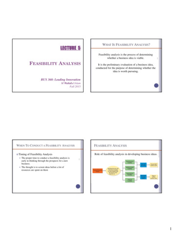
RAn Ethanol Plant in Missouri.Source: J. Marc Raulston.ecent resurgence of interest in ethanolproduction by rural development groups,politicians, and grain producers can beattributed to many different factors such as depressedcommodity prices, rising gasoline prices, shifts inenvironmental policy, and a push towards nationalfuels self-sufficiency. Grain producers in manyregions are considering the development of ethanolplants to help overcome low crop prices. Bryan andBryan International (2006) report that in 2005 therewere 95 ethanol plants in the US with a combinedproduction capacity of 4,336 MMGPY1. Kenkel andHolcomb (2006) expect the trend of privately ownedplants to continue as plants expand into feedstockdeficit regions.Expansion to feedstock deficit regions will likelyreduce the profitability of ethanol plants as feedstockcosts increase and also will likely increase their risk.Like all agribusinesses, ethanol plants face the fullrange of risk on economic variables, such as: inputprice, product price, fuel costs, rate of inflation,and interest rates. The price of the feedstock foran ethanol plant is dependent upon national andinternational supply and demand conditions so itis certainly subject to risk. The price of ethanol hasranged from less than a dollar a gallon two yearsago to over 3.60 per gallon in 2006, demonstratinga significant amount of variability. The price of fuel(natural gas and electricity) used by an ethanolplant has also experienced considerable variabilityover the past few years. Due to the risk faced byan ethanol plant, a comprehensive feasibility studyshould explicitly consider the risk for inputs, suchas: corn, electricity, natural gas, production costs,and operating interest rate; and the risk for outputprices, such as: ethanol and dry distillers grains(DDGS).The literature on ethanol plants and productioncontains numerous examples of feasibility studiesthat ignore risk, e.g. Bryan and Bryan International(2001), Van Dyne (2002), Long and Creason (1997),Whims (2004), Tiffany and Eidman (2003), Shapauri,et al. (2002), and Fruin, et al (1996). Gill (2002) andHerbst (2003) both incorporated risk into ethanolplant feasibility analyses. Failure to incorporateinput cost and output price risk tends to misleadpotential investors and policy makers interestedin helping grain producers through investment inethanol plants.The objective of this study is to demonstratethe benefits of quantifying the economic viabilityof a proposed agribusiness under risk relative to a
feasibility study which ignores risk. To achieve thisobjective, the economic viability of a 50 MMGPYethanol facility in Texas is analyzed over a 10-yearperiod in two ways: with no risk and with historicalrisk for prices and costs.Review of LiteratureMuch of the ethanol literature comes from the1980’s, a boom period for development of ethanolplants, and from the current era, namely 2002 topresent. Topics covered in the literature range fromthe structure of the industry, production technology,ethanol policy, feasibility studies, economic impactstudies, and economies of scale (Van Dyne (2002),Bryan and Bryan International (2001, 2003, 2006),Long and Creason (1997), Gill (2002), Herbst (2003),Tiffany and Eidman (2003), Shapauri, et al. (2002),Whims (2004), and USDA (2006)).The use of ethanol as a fuel additive for internalcombustion engines dates back to the 1920’s, whenStandard Oil marketed, what in today’s notationwould be, E25 (gasoline with 25-percent ethanol,by volume) in the Baltimore area. In 1938, an 18MMGPY alcohol plant was constructed and operatedin Atchison, Kansas, supplying over 2,000 servicestations across the Midwest. After WWII, effortsto sustain U.S. ethanol production failed with theincreased availability of less expensive fuels derivedfrom petroleum and natural gas (DiPardo, 2001).Most all economic feasibility studies for proposedethanol plants ignore price and cost risk. For example,a recent study by Bryan and Bryan International(2001) analyzed the economic viability of a 15MMGPY facility in Dumas, Texas, and included theoperational and construction costs for additionalfacility sizes, including 30 and 80 MMGPY facilities.However, like other ethanol feasibility studies, theyignored ethanol and DDGS price risk and simplyincreased their assumed prices received at a fixedrate of inflation over time2. Risk on corn price andenergy cost was ignored in their study and operatingcosts were simply indexed up over the study period toaccount for inflation. USDA (2006) recently analyzedthe economic feasibility of ethanol production fromseveral feedstocks without incorporating the effectsof price and cost risk.In contrast to other ethanol plant feasibilitystudies, Gill (2002) and Herbst (2003) incorporatedprice and cost risks into their studies. TheirAn Ethanol Plant in Brazil.Source: James Richardson.feasibility studies incorporated price and cost riskby simulating spreadsheet feasibility models usingMonte Carlo techniques. Gill’s (2002) emphasis wason analyzing the economic viability of ethanol plantsfor alternative levels of state subsidies for ethanolproduction in Texas. Herbst (2003) estimated theeconomic variability of ethanol production if theplants used corn vs. sorghum and were located indifferent regions of Texas. Due to incorporatingrisk into their studies, the results were presentedin terms of the probability that the firm will be aneconomic success and the probability of annual cashflow deficits.MethodologyOver the past 10 years there has been aresurgence in the interest in Monte Carlo simulation(Richardson (2006), Winston (1996), and Vose(2000)). The reduced cost of computers, wide spreaduse of Excel and the availability of simulation addins for Excel has made this methodology affordableto business. Monte Carlo simulation offers business
analysts and investors an economical means ofconducting risk-based economic feasibility studiesfor new investments and a non-destructive means ofstress testing existing businesses.Pouliquen (1970) defines the benefits of stochasticsimulation as providing decision makers the extremevalues for KOVs of interest and their relative probabilitieswith a weighted estimate of the relationships betweenunfavorable and favorable outcomes. In addition to theanalysis of risk and how it affects the feasibility of aproject, Pouliquen (1970) suggested that the completedfeasibility simulation model can be used to analyzealternative management plans if the investment isundertaken.Richardson (2006) outlines the steps for developinga production-based investment feasibility simulationmodel. First, probability distributions for all riskyvariables need to be defined, parameterized, simulated,and validated. Secondly, the stochastic values from theprobability distributions are linked to the accountingrelationships needed to calculate production, receipts,costs, cash flows, and balance sheet variables for theproject. Stochastic values sampled from the probabilityStochastic SimulationIgnoring risk in the feasibility analysis of aproject only provides a point estimate for key outputvariables (KOVs) instead of probability distributionsthat show the risks of success and failure (Pouliquen(1970), Reutlinger (1970), and Hardaker, et al.(2004)). Following the examples of Richardson andMapp (1976), Pouliquen (1970), Reutlinger (1970),and Richardson (2006), a stochastic simulation modelof a proposed ethanol production facility in Texas isdeveloped and applied to demonstrate the benefitsof Monte Carlo simulation for feasibility studies ofagribusinesses.An Ethanol Plant in Iowa.Source: George Knapek.
distributions thus make the financial statementvariables stochastic. By stochastically samplingthe probability distributions many times (say, 500iterations) the model generates empirical estimates ofprobability distributions for unobservable KOVs suchas present value of ending net worth, net present value,and annual cash flows, so investors can evaluate theprobability of success for a proposed project.Due to the annual nature of grain feedstocks foran ethanol plant, the Monte Carlo feasibility model isan annual model. In addition to the stochastic variablepart of the model, it has all of the accounting equationsfor an income statement, a cash flow statement, and abalance sheet. The parts of the model are described inthe following sections.forecasted value. The random components of PPI andinterest rates were the residuals from their meanexpressed as a fraction of the means. The local pricesof corn in Texas were simulated by adding a stochasticwedge to national corn prices based on the historicaldifference between national and state annual averageprices. The correlation matrix used to simulate the MVEdistribution for the random variables was calculatedusing the unsorted residuals from trend or mean.Projected means for the stochastic variables overthe 2006-2015 study period came from several sources.Projected annual prices for corn, DDGS, interest ratesand PPI rates of inflation came from the January 2006FAPRI Baseline. Annual average prices for electricity,gasoline, and natural gas were projected using their2005 prices and FAPRI’s projection for annual ratesof change in the prices of fuel. Annual average pricesfor ethanol were assumed to be either 1.80/ gallon, 2.20/ gallon, or 2.50/gallon throughout the planninghorizon. The pessimistic price projection of 1.80/gallonis slightly higher than the average price in 2004 of 1.72. The optimistic price scenario of 2.50/ gallonis consistent with prices the first half of 2006, whilethe 2.20/gallon represents a more moderate priceprojection.Stochastic VariablesStochastic variables in the ethanol model are annualprices for: corn, ethanol, dry distillers grain (DDGS),electricity, natural gas, gasoline, operating interestrate, and inflation rate on production costs. Ethanoland DDGS prices affect cash receipts while the otherstochastic variables affect costs of production and all ofthese variables affect net cash income, cash reserves,net worth, and ultimately net present value.The stochastic variables were simulated using themultivariate empirical (MVE) distribution (Richardson,Klose and Gray, 2000) to account for the correlationamong the variables. Historical data for the 1989-2005period were used to estimate the parameters for theMVE distribution. Parameters for the MVE distributionare: deviations from mean or trend expressed as afraction (the stochastic component), correlation matrix(the multivariate component), and the projected meansfor the 10 year planning horizon (the deterministiccomponent).Historical corn and DDGS prices were obtainedfrom the United States Department of Agriculture(USDA), Economic Research Service, Feed Grains DataDelivery Service for 1989 through 2005. Ethanol priceswere collected from Hart’s Oxy-Fuel News from 1989 to2005. Historical annual gasoline, industrial electricity,and natural gas prices were obtained from the UnitedStates Department of Energy. Historical operatinginterest rates and the index of prices paid (PPI) wereobtained from FAPRI.The stochastic components for ethanol, DDGS,corn, gasoline, natural gas, and electricity were theirresiduals from trend expressed as a fraction of theThe Economic ModelPro forma financial statements in the economicmodel link the annual stochastic variables to assumedproduction and cost coefficients for simulating annualcash flows and net present value over a 10 year planninghorizon. The following sections describe the pro formafinancial statements and the order of calculations inthe economic model.Income StatementTotal annual receipts were calculated by summingthe stochastic annual ethanol and DDGS receipts andinterest earned on ending cash balances. Receipts forethanol equals production times the stochastic price ofethanol.The plant is projected to run half of the first yearand near full capacity in the remaining years of theplanning horizon (plus five percent denaturant).Because of stochastic down time for maintenance,the plant will not run at 100 percent capacity. Toaccount for the stochastic down time, the productioncapacity was adjusted using a GRKS distribution3.
The GRKS distribution used a minimum days down of10 and a maximum of 20 with a middle value of 15;these parameters were reduced 50% for the first year.Corn used by the plant equaled stochastic productiondivided by 2.75 gallons per bushel4 so corn purchasedis a stochastic variable. Annual DDGS receipts werecomputed by multiplying quantity of corn purchasedby the DDGS per bushel of corn coefficient, 18 lbs/bushel5, and the DDGS stochastic price. Interestearned on beginning year cash balances was includedin the income statement and was calculated using thestochastic operating interest rate minus the historicaldifference between savings and operating interest ratestimes the positive cash balances.The cost of corn used for the fermentation processwas the product of the stochastic price of corn andthe stochastic quantity of corn purchased. Per gallonvariable production costs for the first year ( 0.93/gallon) come from a recent BBI (2003) plant handbookIowa corn.and were inflated using stochastic annual inflationrates, and multiplied by the volume of anhydrousethanol produced per year to compute total variablecosts6. Electricity and natural gas costs were calculatedbased on input requirements for a 50 MMGPY plant(BBI, 2003) and the stochastic annual prices for theseinputs7. Start-up expenses of buying initial inventoriesof supplies and corn along with the cost of hiring andtraining employees was included at 9 million.Total annual costs were computed by summingannual corn costs, variable costs, electricity and naturalgas costs, loan interest costs, and deprecation expense.Depreciation expense was calculated using MACRS onthe plant, annual capital improvements, and capitalizedstart up costs. Net income (losses) equaled the totalannual receipts minus total annual costs.Matt Sederstrom (2006) of Fagen, Inc. reportedthat the cost to build a 50 MMGPY plant requires 1.75 per gallon of capacity. The 95 million of capitalSource: George Knapek.
The probability of economic success was calculatedusing the net present value (NPV):includes construction and land costs. The presentanalysis assumed that 50 percent of the total capitalrequirements were borrowed and the remaining 50percent were contributed by owner/investors. The 8year loan on the plant was amortized using a fixedinterest rate of 9.5 percent.An operating loan equal to 15 percent of total annualvariable costs was used in the model and the cost ofthe loan was calculated using a stochastic interest rate.Stochastic operating interest rates were used for shortterm loans to finance cash flow deficits over the 10 yearanalysis period.10 Dividendst AnnualNetWorthtNPV BeginningEquity (1 0.25)tt 1 If the NPV is positive, the firm has a rate of returngreater than the discount rate, i, or 0.25, and is consideredto be an economic success (Richardson and Mapp,1976). In stochastic simulation, the model recorded aone for iterations when the firm had a positive NPV anda zero otherwise. The probability of economic successwas calculated as the sum of 1’s for the NPV countervariable divided by the number of iterations.Cash Flows StatementModel AssumptionsBeginning cash equaled the positive ending cashbalances in the balance sheet from the previous year.In year one beginning cash balance was zero for theplant. The sum of annual beginning cash balance andnet cash income (plus depreciation) equals total annualcash inflows. Annual cash outflows were calculated bysumming the principal payments for the initial capitalloan, repayments of cash flow deficits, income taxes anddividends.A corporate business structure was assumed whencalculating federal income taxes for the proposed plant.For the purposes of this study, 35 percent of positivenet income is paid as a dividend each year8. Total cashinflows minus annual total outflows equaled ending cashbalance before borrowing. If the ending cash balancewas negative, then the firm must borrow funds to makeending cash balance equal zero. Loans to cover cashflow deficits were assumed to be one year extensionsof the operating loan and must be fully repaid the nextyear.The assumptions used in the model to simulate a 50MMGPY ethanol plant are summarized in this section interms of a gallon of ethanol produced. Ethanol yields 2.75gal/bu of corn, DDGS yields 18 lb/bu of corn, and variablecosts were: denaturant (gasoline) 0.0762/gal, enzymescost 0.04/gal, chemicals cost 0.04/gal, maintenancematerials 0.02/gal, labor 0.05/gal, and miscellaneousand water treatment costs 0.03/gal (BBI 2003). Toincorporate the effect of an uncertain rate of inflationfor variable costs, the initial costs were inflated eachyear using stochastic inflation rates. Natural gas andelectricity costs per gallon were simulated using theirrespective stochastic prices and energy requirementsof 0.038MCF/gal and 0.80 Kwh/gal, respectively (BBI,2003). Capital requirements including construction andstartup costs are 87.5 million (Sederstrom, 2006), andannual capital replacement costs totaling 875,000, or 1percent, per year. It was assumed that the 50 MMGPYfacility would be operated at half of year 1 and 100percent of capacity in years 2-10 for the deterministicmodel and stochastically it will operate at half capacityin year 1 and about full capacity in years 2-10.All of the input/output coefficients were the samefor the deterministic and the Monte Carlo feasibilityanalyses. The annual values for all stochastic variableswere held constant at their mean values in thedeterministic analysis.A minimum ethanol price of 1.80 was assumed inthe model and a minimum wholesale gasoline price of 1.25 was assumed. The minimums were used to reflectthe recent prices for petroleum and ethanol.The model described in this section was programmedin Microsoft Excel using standard accounting identitiesand equations. The financial model was made stochasticBalance SheetValue of total assets was calculated annually usingending cash balances, land value9, and book valuefor plant, and equipment adjusted for the MACRSdepreciation table for a 15-year recovery period(Smith, et al., 1998). Total liabilities equaled long-termliabilities (the current ending balance of the originalloan) plus current year cash flow deficits. Net worthwas computed by subtracting total liabilities from totalassets. Net worth is used in two forms: a) nominal orcurrent dollar terms, and b) real dollars, for which thenominal values have been discounted using a discountrate of 25 percent.
Table 1: Results of Deterministic and Stochastic Ethanol Plant Models for Three AssumedEthanol Price Scenarios. 1.80/GallonDeterministic ModelPVENW (mil s)NPV (mil s)ROI (%)Variable Cost in 2007 ( /gallon) 2.20/Gallon 42.79127.4670.61.2158Monte Carlo Feasibility ModelPVENWMean (mil s)Standard Deviation (mil s)Coefficient of Variation (%)Minimum (mil s)Maximum (mil .773.027.2329.8350.74Net Present Value (NPV)Mean (mil s)Standard Deviation (mil s)Coefficient of Variation (%)Minimum (mil s)Maximum (mil .96122.0715.4912.6967.95161.69Return on Investment (ROI)Mean (%)Standard Deviation (%)Coefficient of Variation (%)Minimum (%)Maximum 5792.546.785.3Variable Costs in 2007Mean ( /gallon)Standard Deviation ( /gallon)Coefficient of Variation (%)Minimum ( /gallon)Maximum ( .446.8010046.8010046.8Prob (NPV 0) (%)Prob (Economic Success) (%)Prob (Stoch VC Deter VC)using Simetar , an add-in for Excel (Richardson,Schumann and Feldman, 2006). Simetar was used toestimate the parameters for the multivariate empiricalprobability distribution, and Simetar simulated themodel using a Latin hypercube sampling procedure forsampling random variables.summarized in Table 1. The results were presentedin terms of the present value of ending net worth(PVENW), the net present value (NPV), variable costsper gallon and the probability of economic success. Thefeasibility of the plant was tested under three differentethanol price scenarios. The annual mean prices usedfor Scenarios 1 - 3 were, respectively, 1.80/gallon, 2.20/gallon, and 2.50/gallon of ethanol.The cost of production did not change withscenarios. The deterministic variable cost per gallonof ethanol with credits for DDGS was 1.216 inResultsResults of the economic feasibility analysis for a 50MMGPY ethanol plant in the Texas Panhandle were
0.750.951.151.35 /gallon1.551.751.95Figure 1: Probability Density Function of the Variable Cost per Gallons of Ethanol, with DDGSCredit for (2007).-50.000.0050.00100.00150.00200.00Mil. sNPV: 1NPV: 2NPV: 3Figure 2: The Probability Density Functions of NPV for Scenarios 1, 2 and 3.Deterministic NPVs for Scenarios 1, 2, and 3, were 8.71, 76.62, and 127.46 million, respectively.Rate of return on investment (ROI) was 26.5, 51.7,and 70 percent for the three scenarios.The Monte Carlo feasibility study resulted inaverage PVENW values that were similar to thedeterministic study for all three price scenarios;however, the risk analysis produced estimatesof the variability on PVENW, NPV, and ROI. ForScenario 1, the deterministic PVENW was 17.25million and the risk study reported a mean PVENWof 20.03 million. The NPV for the deterministicand stochastic analysis were 8.71 million and 20.94 million, respectively, for Scenario 1 andthe stochastic analysis projected NPV would have2007. The stochastic average variable cost per gallonwas 1.219, with a standard deviation of 0.144and a coefficient of variation (CV) of 11.81 percent.The minimum and maximum variable costs were 0.912 and 1.769, respectively. Figure 1 presentsthe probability density function (PDF) chart of thevariable cost in 2007 for the stochastic scenarios. Thedeterministic cost of production (the vertical line at 1.21/gallon in Figure 1) is 52 cents less than themaximum and 30 cents greater than the minimumdue to the skewed nature of production costs.Based on the assumptions for the 50 MMGPYplant a deterministic feasibility study would reportPVENW values of 17.25, 31.89, and 42.79 millionfor ethanol price Scenarios 1, 2, and 3, respectively.
0140160180Mil. sNPV: S1NPV: S2NPV: S3NPV: D1NPV: D2NPV: D3Figure 3: The Cumulative Distribution Functions for the Deterministic and Stochastic results for Scenarios 1, 2 and 3.a minimum and maximum of - 5.87 million and 46.86 million, respectively. By only analyzing thedeterministic NPV, one misses the range of possibleoutcomes and could make a bad business decision.For Scenario 2 ( 2.20/gal), the PVENW for thedeterministic analysis was 31.89 million and 31.27million for the Monte Carlo analysis. The NPV forthe deterministic and stochastic studies were 76.62million and 73.14 million, respectively, and thestochastic analysis has a minimum and maximumNPV of 26.33 million and 106.96 million,respectively, for an 80 million range.Under Scenario 3 ( 2.50/gal) the PVENW forthe deterministic study was 42.79 million and 41.77 million for the stochastic model. The NPVfor the deterministic results was 127.46 millionand 122.07 million for the stochastic analysis andthe stochastic minimum and maximum NPVs were 67.95 million and 161.09 million, respectively fora 93 million spread.The simulation risk analysis showed an averageROI for Scenario 1 of 31.3 percent, slightly higherthan the deterministic ROI of 26.5 percent (Table1). For Scenarios 2 and 3 the average ROI from therisk analysis was 50.7 and 68.8 percent, both lessthan there respective deterministic results. Moreimportantly the risk analysis indicated that investorscould expect considerable variability in ROI. UnderScenario 2 the ROI could range from 31.5 percent to64.9 percent with a 55 percent chance of the ROIsexceeding 50 percent. Under Scenario 1 there wasa 34 percent chance that ROI would be less than 30percent.By examining the simulated values for NPVover all iterations simulated, the model indicatedthe probability that NPV would be negative. ForScenario 1 the probability of a negative NPV was1.6 percent (Table 1). For Scenarios 2 and 3 theprobability of a negative NPV equaled zero. As aresult the probability of economic success is 98.4percent for Scenario 1 and 100 percent for Scenarios1 and 3, based on the probability of returning areturn greater than the 25 percent discount rate.Figure 2 presents the probability density function(PDF) charts of NPV distributions for the threestochastic scenarios and the deterministic NPV forthe no-risk scenarios. The deterministic NPVs aredepicted as vertical lines in the three PDFs. Theassumption that ethanol price has a minimum of the 1.80/gal is responsible for the narrow dispersion ofthe PDF for Scenario 1.Figure 3 presents a cumulative distributionfunction (CDF) chart of the simulated NPVdistributions under the three price scenarios. Thethree vertical lines in the CDF chart represent thedeterministic NPVs for the three scenarios. The line
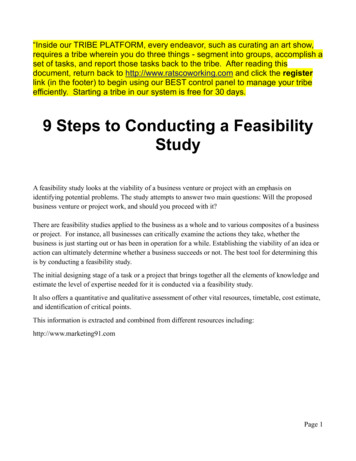
706050Mil. s403020100-1020062007200820092010201125th PercentileAverage5th PercentileFigure 4: A Fan Graph of Annual Net Cash Income for Scenario 2for the deterministic NPV crosses the CDF for itsassociated stochastic scenario at different points foreach scenario. Scenario 1’s deterministic NPV crossesthe CDF at the 10 percent level because there is anassumed minimum price for ethanol of 1.80 and thesimulated ethanol price does not fall below 1.80. InScenarios 2 and 3 the deterministic NPV line crossesthe associated CDF at approximately the 60 percentlevel indicating that the deterministic analysis hasa positive bias. The probability distributions and theCDFs for NPV generated by the Monte Carlo modelprovide a great deal more information about theeconomic viability of the proposed business than thedeterministic analysis.Figure 4 presents a fan graph of the annual netcash income (NCI) under Scenario 2 for the 10-yearplanning horizon. The fan graph illustrates the rangeof possible NCI for each year of the planning horizon.The top line represents the 95-percentile line whilethe bottom line represents the 5-percentile line. Thismeans 90 percent of the time annual NCI falls betweenthese lines so the two lines represent a 90 percentconfidence interval for NCI in each year. The middleline is the average. The lines second from the bottomand top represent the 25 percentile and 75 percentilelines, respectively; so they represent the 50 percentconfidence interval for annual NCI. The fan graphshows a positive trend in NCI and has relatively little201275th Percentile20132014201595th Percentilechange in the overall NCI variability over the 10-yearperiod. Figure 5 presents a fan graph of the EndingCash for Scenario 2 over the 10-year planning horizonand shows a positive trend in cash reserves but withincreasing variability over time.ConclusionsThe purpose of this paper was to demonstrate theusefulness of Monte Carlo simulation for evaluatingthe economic viability of a proposed agribusiness.A simulation model of a 50 MMGPY ethanol plantin the Texas Panhandle was developed based onaccepted input/output coefficients and investmentcosts. Stochastic values for costs and prices wereincorporated into the model using historical risk forthese variables, thus facilitating a simulation riskanalysis of the business.The simulation model was developed usingstandard accounting principles and pro formafinancial statements. Key output variables for theanalysis were variables of interest to potentialinvestors, namely: present value of ending net worth(PVENW), net present value (NPV), rate of return toinvestment (ROI), probability of economic success,and annual cash flows. Additional output variablesof interest to investors, such as financial ratios, canbe reported for a Monte Carlo simulation model.10
200180160Mil. 201220132014201575th Percentile25th Percentile5th Percentile95th PercentileFigure 5: A Fan Graph of Annual Ending Cash for Scenario 2.To demonstrate the usefulness of simulation riskanalysis the results of three alternative scenarioswere reported for a proposed ethanol plant. Thepro forma financial statement simulation modelwas run two ways: deterministic and stochastic.The same parameters for the plant and means forthe stochastic costs and prices were used for bothmethodologies. Both the determinist
resurgence in the interest in Monte Carlo simulation (Richardson (2006), Winston (1996), and Vose (2000)). The reduced cost of computers, wide spread use of Excel and the availability of simulation add-ins for Excel has made this methodology affordable to business. Monte Carlo simulation offers business An Ethanol Plant in Brazil.