Transcription
TR-88 — Task Force on Dynamic State and Parameter EstimationIEEE Task Force onDynamic State and Parameter EstimationChair: Junbo Zhao, Mississippi State University, USAVice-Chair: Alireza Rouhani, Dominion Energy, USASecretary: Shahrokh Akhlaghi, Southwest Power Pool, USAMembers (Alphabetical Order):xxxxxxxxxxxxxxxxxxxxAbhinav Kumar Singh, University of Southampton, U.K.Abdul Saleem Mir, University of Southampton, U.K.Ahmad Taha, University of Texas at San Antonio, USA.Ali Abur, Northeastern University, USA.Antonio Gomez-Exposito, University of Seville, Spain.A. P. Sakis Meliopoulos, Georgia Institute of Technology, USA.Bikash Pal, Imperial College London, U.K.Innocent Kamwa, Laval University, Canada.Junjian Qi, Stevens Institute of Technology, USA.Lamine Mili, Virginia Polytechnic Institute and State University, USA.M. A. M. Ariff, Universiti Tun Hussein Onn Malaysia, Malaysia.Marcos Netto, National Renewable Energy Laboratory, USA.Mevludin Glavic, Independent Researcher, Bosnia and Herzegovina.Samson Shenglong Yu, Deakin University, Australia.Shaobu Wang, Pacific Northwest National Laboratory, USA.Tianshu Bi, North China Electric Power University, ChinaThierry Van Cutsem, University of Liège, Science, Belgium.Vladimir Terzija, Skolkovo Institute of Science and Technology, Russia.Yu Liu, ShanghaiTech University, China.Zhenyu Huang, Pacific Northwest National Laboratory, USA.
TR-88 — Task Force on Dynamic State and Parameter EstimationACKNOWLEDGMENTSThe Task Force is truly grateful for the support of our sponsoring committee on PowerSystem Operations, Planning and Economics Committee, and Bulk Power SystemOperations subcommittee.The Task Force gratefully acknowledges the contributions of participants of our Task ForceMeetings who contributed through their discussions in converging on this report.KEYWORDSBad data, converter-based resources, Energy Management Systems, Dynamic stateestimation, Forecasting-aided state estimation (FASE), Frequency stability, Kalman filter,Parameter estimation, Power system stability, Power system state estimation, Powersystem control, Power system protection, Power system operation, Power systemmodeling, Renewable energy, Robust estimation, State Estimation, Synchrophasormeasurements, Sampled value measurements, Static state estimation (SSE), Tracking stateestimation (TSE), Voltage stability.
TR-88 — Task Force on Dynamic State and Parameter EstimationCONTENTS TF Objectives . 1 TF Background. 1 Power System Dynamic State Estimation: Motivations, Definitions and Methodologies . 2 3.1 Motivations of DSE . 2 3.2 Unified State Estimation Framework . 4 3.2.1 Quasi-Steady State versus Transient Operating Conditions. 4 3.2.2 Dynamic State Estimation . 6 3.2.3 Forecasting-Aided State Estimation . 7 3.2.4 Tracking State Estimation . 7 3.2.5 Static State Estimation . 8 3.3 Tools and Methods for Implementation of DSE . 8 3.3.1 Observability Analysis for DSE . 8 3.3.2 Implementations of DSE . 10 3.3.3 Parameter Estimation and Calibration using DSE . 13 3.3.4 Centralized vs. Decentralized DSE . 13 3.4 Conclusions and Outlook . 14 Roles of DSE in Power System Modeling, Monitoring and Operation . 16 4.1 Introduction. 16 4.2 Comparisons with SSE and DSE . 18 4.2.1 Implementation Differences . 18 4.2.2 Functional Differences . 20 4.2.3 Practical Implementation of DSE . 21 4.3 DSE for Modeling, Monitoring and Operation . 22 4.3.1 Modeling. 22 4.3.2 Monitoring . 24 4.3.3 Operation . 27 4.3.4 DSE for Power Electronics-Interfaced Renewable Generation Visibility. 29 4.4 Conclusions and Outlook . 30 DSE for Power System Control and Protection . 31 5.1 Introduction. 31 5.2 DSE Formulation: Sampled Value Measurements versus PMU Measurements . 32
TR-88 — Task Force on Dynamic State and Parameter Estimation5.3 Controller Options: DSE versus Observer. 34 5.4 Control Applications of DSE. 35 5.4.1 DSE-Based Control using PMU Measurements . 36 5.4.2 DSE-based Control using SV Measurements . 43 5.5 Protection Applications of DSE . 44 5.5.1 DSE-based Protection using PMU Measurements . 44 5.5.2 DSE-based Protection and Fault Location Using SV measurements . 46 5.6 Conclusions and Outlook . 48 Demonstrative Examples . 51 6.1 DSE-based Protection Using SV Measurements . 51 6.1.1 System Description . 51 6.1.2 Test Cases and Results . 52 6.1.3 Summary. 60 6.2 DSE-based Adaptive-Phasor Approach to PMU Measurement Rectification for LFODEnhancement . 61 6.2.1 Overview of DSE Adaptive-phasor-based Data Recovery Method . 61 6.2.2 Case study and simulation results . 62 6.2.3 Summary. 66 Conclusion 66 References66 APPENDIX 80 IEEE PES Webinar Session on DSE Questions and Answers . 80
TR-88 — Task Force on Dynamic State and Parameter EstimationTF ObjectivesThis report of TF on dynamic state and parameter estimation aims to 1) review itsmotivations and definitions, demonstrate its values for enhanced power systemmodeling, monitoring, operation, control, and protection as well as power engineeringeducation; 2) provide recommendations to vendors, national labs, utilities and ISOs onthe use of dynamic state estimator for enhancement of the reliability, security, andresiliency of electric power systems.TF Background and AchievementsThe widespread deployment of phasor measurement units (PMUs) on powertransmission grids has made possible the real-time monitoring and control of powersystem dynamics. However, these functions may not be reliably achieved without thedevelopment of a fast and robust dynamic state estimator (DSE). Indeed, the estimatedsynchronous machine state variables can be used by power system stabilizers,automatic voltage regulators, and under-frequency relays to enhance small signalstability and to initiate generation outages and load shedding during transientinstabilities, etc. During the 2017 IEEE Power Engineering Society General Meetingheld at Chicago, the Working Group on Power System Static and Dynamic StateEstimation decided to form a new task force on “Power System Dynamic State andParameter Estimation” to define its concepts, demonstrate its values for enhancedpower system modeling, monitoring, operation, control, and protection as well as powerengineering educations.Thanks to the dedicated efforts by all TF members, this TF has made the followingcontributions:xThree TF papers published in the IEEE Transactions on Power Systems:-Y. Liu, A. K. Singh, J. B. Zhao, A. P. Meliopoulos, B. Pal, M. A. M. Ariff, T. VanCutsem, M. Glavic, Z. Huang, I. Kamwa, L. Mili, A. Saleem Mir, A. Taha, V.Terzija, S. Yu, "Dynamic State Estimation for Power System Control andProtection," IEEE Trans. Power Systems, 2021.-J. B. Zhao, M. Netto, Z. Huang, S. Yu, A. Exposito, S. Wang, I. Kamwa, S.Akhlaghi, L. Mili, V. Terzija, A. P. Sakis Meliopoulos, B. Pal, A. K. Singh, A.Abur, T. Bi, A. Rouhani, ''Roles of Dynamic State Estimation in Power SystemModeling, Monitoring and Operation," IEEE Trans. Power Systems, vol. 36, no. 3,pp. 2462-2472, 2021.-J. B. Zhao, A. Exposito, M. Netto, L. Mili, A. Abur, V. Terzija, I. Kamwa, B. Pal,A. K. Singh, J. Qi, Z. Huang, A. P. Sakis Meliopoulos, ''Power System DynamicState Estimation: Motivations, Definitions, Methodologies and Future Work,"IEEE Trans. Power Systems, vol. 34, no. 4, pp. 3188-3198, 2019. (Highly CitedPaper according to Web of Science since March 2021)xInvited IEEE PES webinar sponsored by IEEE Transactions on Power Systemsentitled “Dynamic State and Parameter Estimation for Power System1
TR-88 — Task Force on Dynamic State and Parameter EstimationxxMonitoring, Modeling, Operation, Control, and Protection” on 11:00 AM-1:00pm US ET/8:00 AM-10:00 AM US PT, 6th, Friday, November 2020.Tutorial at the 2019 IEEE PES General Meeting entitled “Dynamic StateEstimation for Power System Dynamic Monitoring, Protection and Control:Motivations, Tools and Experiences” Sunday, August 4, 8:00 AM – 5:00 PM.Organized three panel sessions at IEEE PES General Meetings:- “Advanced Dynamic State Estimation for Next Generation of EMS: Structure,Algorithms and Experiences” at IEEE PES General Meeting, DC, 2021.-State Estimation for Power Electronics-Dominated Systems: Challenges andSolutions” at IEEE PES General Meeting, Canada, 2020.-“Dynamic State Estimation for Power System Monitoring, Protection andControl–Paving the Way for A More Resilient Grid” at IEEE PES GeneralMeeting, Atlanta, 2019.Power System Dynamic State Estimation: Motivations,Definitions, and MethodologiesIn this Section, DSE is presented in a unified framework, which uses commonlyaccepted notations and formulations in power system dynamics and control literatureto establish a firm baseline for future research and development efforts. The similaritiesand differences between DSE and other existing estimation methods, includingforecasting-aided state estimation (FASE), tracking state estimation (TSE) and staticstate estimation (SSE), are clarified. Potential applications of DSE are identified anddiscussed to justify its significance for enhanced monitoring, protection, and control.3.1Motivations of DSEPower systems are planned to be operated and controlled in a hierarchical manner [1].The controls are particularly designed to deal with a variety of dynamic phenomena atmultiple time scales [2]. For example, a synchronous generator's automatic voltagecontrol is based on locally available measurements only. However, their voltage setpoints can be modified when the command from the centralized control center isreceived. Hence, there exists a hierarchical decentralized closed-loop control thatresponds to system variations and to set point changes. The centralized open-loopcontrol is triggered by the operator after a decision-making process. Following thisphilosophy of design, most of the monitoring and control applications at the controlcenter rely on the steady-state model of the system. However, in the real world, powersystems never operate in a steady-state condition, as there are stochastic variations indemand and generation. The situation is further aggravated by the large-scaleintegration of distributed energy resources (DERs) on the generation side, and complexloads and new demand-response technologies on the demand side, such as electricvehicles and internet of things devices. Such a shift has given rise to larger uncertaintiesof the system's dynamic characteristics. Consequently, the steady-state assumptionbecomes questionable, and SSE methods are unable to capture these dynamics in anoperational environment. As a result, SSE methods [3]-[6] used in today's energymanagement systems (EMS) should be reassessed and enhanced with new monitoringtools, such as DSE. DSE is capable of accurately capturing the dynamics of the systemstates and will play an important role in power system control and protection [7]-[11],especially with the increasing complexity resulting from the uncertainties by the newtechnologies being deployed in the generation and demand sides.2
TR-88 — Task Force on Dynamic State and Parameter EstimationWith the widespread deployment of PMUs and advanced communication infrastructurein power systems [12], [13], the development of a fast and robust DSE tool has becomepossible. The benefits of using DSE include but are not limited to:x Improved oscillations monitoring: the estimated dynamic state variables can beused to carry out modal analysis [14], and the identified modes can then beutilized to adaptively tune power system stabilizers (PSS), thereby achievingbetter damping of inter-area modes of oscillation and improving systemstability. Recall that the effectiveness of conventional PSS using localmeasurements may be limited by the observability of the modes in the signal.Using state estimates of entire regions as opposed to only local measurementswill increase the stabilizer's response to inter-area modes if the generator has asignificant influence on such modes. Note that there are several ways formonitoring the entire regions/systems via DSE, namely the hierarchical anddistributed DSE and the centralized DSE using high-performance computingtechnique [15], [16], or reduced-order model of power system [17]. Hierarchicaland distributed DSE methods are first implemented locally to monitor smallareas, and their results are submitted to the control center for further processing.This is the widely used strategy in the current literature. The DSE based on highperformance computing for large-scale systems is in its infancy, and meritsfurther research;x Enhanced hierarchical decentralized control [18]-[20]: the availability of localand wide-area dynamic states obtained from DSE enables the design of effectivelocal and wide-area controls; for instance, the estimated rotor speed and otherstates can be used as input signals to control excitation systems of synchronousmachines [19], [20] or of FACTS devices [18] to damp out oscillations. Theimplementation can be in either fully decentralized or hierarchicallydecentralized manner;x Improved dependability and reliability of protection systems [8], [21]-[23]: bytesting the consistency between the PMU measurements and the dynamicalmodel of the protection zone for which the parameters are identified by DSE,both internal and external faults can be effectively detected without any a prioriprotection relay settings, yielding more reliable protection systems comparedwith the traditional coordinated settings-based schemes; the dynamic statesestimated online can be utilized to initiate effective generator out-of-stepprotections [11], [23] and transient stability monitoring based on the extendedequal-area criterion or the energy function approach [23]; furthermore, fast stateestimation is a prerequisite for the implementation of system integrity protectionschemes that can prevent blackouts;x Enhanced reliability of the system models utilized for dynamic securityassessment (DSA) [24]: DSA requires the availability of accurate models of thegenerators and their associated controllers, of the composite loads, and thespecial protection schemes, to name a few. By developing DSE, both the staticand dynamic models can be validated [25], and if incorrect parameter values areidentified, they can be included as additional state variables in DSE forparameter estimation and calibration, yielding improved system models [26]and more reliable DSA;x Other applications: improved synchrophasor data quality and cyber securityleveraging the model information, such as filtering out measurement error thatis modeled as Gaussian or non-Gaussian distribution [27], [28], detecting bad3
TR-88 — Task Force on Dynamic State and Parameter Estimation3.2and delayed measurements, or recovering missing data [29]; enhancedsynchronous generators coherency identification and dynamic model reduction[30] using the estimated dynamic states and parameters; enhanced busfrequency and center of inertia estimation [31], [32] and detection of failures incontrollers, such as excitation systems, PSS, etc., [33], [34].Unified State Estimation FrameworkThis section develops a unified framework for various power system state estimationapproaches, namely DSE, FASE, TSE, and SSE. Specifically, the system operatingconditions and the associated mathematical models are first revisited. Then, theresulting state transition expressions are identified and subsequently customized fortransient and quasi-steady-state operating conditions.3.2.1Quasi-Steady State versus Transient Operating ConditionsThe states of a system are essential in any of two mutually exclusive operatingconditions, quasi-steady and transient, see Fig. 1.Fig. 1. Illustration of power system statesThe tutorial example depicted in Fig. 2 is used to illustrate the models and conceptsarising in the discussion. In this simple system, an aggregated load is served both by alocal generator and an external grid represented by its Thevenin equivalent. Slow loadevolutions can be analyzed by solving the system of algebraic equations (see below),while sudden changes, such as opening the CB, call for the solution of differentialequations.4
TR-88 — Task Force on Dynamic State and Parameter EstimationFig. 2. Tutorial exampleFor this particular example, assuming a second-order classical dynamic model for thelocal generator, the system shown in Fig. 2 becomes:Differential equations:2HZ0E 'Vsin (G T )XZPm GZ Z0Algebraic equations:PLE 'VEVsin (G T ) f sin TXXfQLVVE 'cos (G T ) V Efcos T VXXfInput and state vectors:x [G , Z ]Ty [V ,T ]Tu [ PL , QL ]Tp [ X , X f , Pm , H ]TAs far as the system parameters are concerned, they can be classified into the followingcategories: Well-defined (good enough accuracy) and constant parameters (e.g. networkimpedances, generator inertia constant, etc.). These define the coefficients of themodel and do not have to explicitly appear in the functional dependence. Uncertain (constant or time-varying) parameters. These should be included in thestate vector (x or y), to be estimated like any other regular variable (e.g., a lineresistance changing with temperature). Time-varying parameters that evolve in accordance to a given control law orpredefined action, leading to slow or fast dynamic phenomena (e.g., the tap settingof a transformer, the impedance of a shunt compensator, etc.). These should beincluded in the control vector (u).For instance, in the tutorial example, the inertia constant H could be included in thestate vector if one wishes to estimate a better value than that provided by themanufacturer, whereas the mechanical power Pm could be considered an input if thespeed governor dynamics are not included in the model, or a state variable otherwise.5
TR-88 — Task Force on Dynamic State and Parameter EstimationTransient operating condition: arises when a sudden disturbance takes place in thesystem. In this context, only electromechanical transients are considered and theassociated governing equations are those customarily adopted for transient stabilityanalysis, given byx (t ) f ( x (t ), y(t ), u(t ), p), 0 g( x(t ), y(t ), u(t ), p)ximini d xi d ximax , i ; uimin d ui d uimax , j :pimin d pi d pimax , l *(1)where x א Rn represents the system state vector, such as the internal states of a machineor a dynamic load, etc.; y א Rm represents the algebraic state vector, such as voltageand current phasors; note that the algebraic equations include those that are associatedwith the power flows and generators’ stator; u is the system input vector; p representsthe model parameters; and f and g are nonlinear functions; due to physical limitations,controller design, some dynamic state variables, control inputs and model parametersare bounded by their upper and lower limits, which are represented by thesets Ȅ, ȍ, and ī, respectively.Quasi-steady state operating condition: refers to the situation in which the systemoperating point changes exclusively due to slow and smooth load/renewable generationchanges. In this scenario, the generators and other controllers can almost instantlyabsorb these slow changes, yielding negligible changes of the dynamic states x(t), i.e.,xÚ (t) § 0. As a result, the system is mathematically characterized by:0 f ( x (t ), y (t ), u(t ), p),0 g ( x (t ), y (t ), u(t ), p),(2)subject to equality and inequality constraints, where slowly varying voltage phasors,i.e., algebraic state variables, are of interest. Since system inputs are usually notperfectly known and the parameters are always inaccurate to a certain extent, stateestimators capable of processing measurement snapshots are developed, includingFASE, TSE, and SSE. It is worth emphasizing that, at the distribution level, individualloads may change abruptly enough for the distributed generators or local controllers tobe subject to disturbances, requiring the dynamic model (1) to be resorted to.In practice, the continuous-time models for both transient and quasi-steady-stateoperating conditions are transformed into their discrete-time state-space forms throughsome time discretization technique [36]. Then (1) can be written asxk0f ( xk 1 , yk 1 , uk , p) wk ,g( xk , yk , uk , p) ek ,(3)(4)where wk and ek are error terms that include time discretization and modelapproximation errors. By treating the equality constraints (4) as pseudo-measurementsand processing them together with the incoming measurements, a more general statespace model for state estimation isxkzkf ( xk 1 , yk 1 , uk , p) wk ,h( xk , uk , p) vk ,6(5)(6)
TR-88 — Task Force on Dynamic State and Parameter Estimationsubject to the constraints defined before, where zk is the measurement vector, includingpseudo-measurements, measured algebraic variables, real and reactive powerinjections, and flows, current phasors, etc.; h is the nonlinear measurement function; vkis measurement error. The wk and vk are usually assumed to be normally distributedwith zero mean and covariance matrices, Qk and Rk, respectively. Note that they are thesuperposition of different sources of noise/errors (e.g. from sensors, communicationchannels, or models) and may not follow a Gaussian distribution in practice.To perform state estimation under the quasi-steady state operating condition, (2) isdiscretized as well, yielding a similar formula as (5) and (6) except for setting xk § xkí1.The use of conventional measurements from remote terminal units is sufficient.Conversely, when the system is operating under transient conditions, synchrophasormeasurements may be the only source of information to carry out DSE. At the locallevel (e.g. generation station, substation, or FACTS device site), digital recorders orprotection devices, also referred to as intelligent electronic devices, can provide therequired synchronized information to execute DSE, possibly including key parametersof the monitored device.Remark: for the existing DSEs, not all the equality and the inequality constraints areduly considered, for example, the inequality constraints of the states, control inputs,and model parameters. The latter may cause serious concerns, such as algorithmdivergence, violation of physical laws, obtaining only sub-optimal solutions, to name afew. Thus, DSE methods that take into account all constraints are needed.3.2.2Dynamic State EstimationTo estimate the dynamic state vector or model parameters of the general discrete-timestate-space model shown in (5)-(6), various nonlinear filters developed within theKalman filter framework are used. It typically consists of two steps [35], namely aprediction step using (5), and a filtering/update step using (6). Specifically, given thestate estimate at time step k-1, xˆ k 1 k 1 , with its covariance matrix, Pk 1 k 1 , the predictedstate vector is calculated from (5) directly or through a set of points drawn from theprobability distribution of xˆ k 1 k 1 , which is dependent on the assumed probabilitydistributions of wk . As for the filtering step, the predictions are used together with themeasurements at time step k to estimate the state vector and its covariance matrix.Depending on how the state statistics are propagated, different Kalman filters areavailable, such as extended Kalman filter (EKF), unscented Kalman filter (UKF),ensemble Kalman filter (EnKF), particle filter (PF) [36], to name a few.The derived state-space equations (5)-(6) allow DSE to be applied rigorously to anypower system, in any condition, provided the available computing power is sufficientfor the size of the problem being addressed and the assumptions that all the equalityand inequality constraints are appropriately enforced. The term 'dynamic', when appliedto a quasi-steady state operating condition may be misleading, as the system dynamicsare actually assumed to be absent/negligible and the state transitions are determinedmainly by the smooth load evolution. In fact, under this scenario, we call the developedestimators either FASE or TSE.Remarks: The state vector can be the enlarged one that contains x and y simultaneously,or the reduced one (x or y), depending on whether algebraic or dynamic states are beingestimated; the state vector x can be expanded to include uncertain parameters of7
TR-88 — Task Force on Dynamic State and Parameter Estimationgenerators and associated controllers. On the other hand, except for the widely usedrecursive estimators that are based on the Kalman filter framework, other non-recursiveestimators can also be adopted for the state and parameter estimation, such as theinfinite impulse response filter, the finite impulse response filter [37], to name a few.3.2.3Forecasting-Aided State EstimationThe so-called FASE is a particular application of the DSE concept to quasi-steady-stateconditions, in which the state-transition model (change in operating point) is drivenonly by slow enough stochastic changes in the power injections (demand andgeneration) and the dynamics of xk are sufficiently small to be neglected. In addition,unlike the original DSE formulation, in the FASE approach, the state-transition model(5) is assumed to be linear, leading toyk Ak yk 1 [ k 1 wk ,(7)zk h( yk , p) vk ,where yk represents the algebraic state variables that specifically refer to the busvoltage magnitudes and angles; furthermore, instead of resorting to the nonlinear statetransition models, the required transition matrix Ak and the trend vector [ k 1 , which isa function of uk , are identified from historical time series data. The widely usedapproaches for that are exponential smoothing regression or recursive least squares[38]-[43]. In other words, the current values are computed from a weighted average ofthe most recent past values, with an exponentially decreasing set of weights,disregarding any other information about the structure of the problem at hand.When the input or the trend vector evolves smoothly, the FASE approach providessatisfactory results, generally better than the simpler TSE. However, potentiallyinaccurate results can be obtained in the presence of sudden changes caused by loads,DERs, system topology, to name a few, as the state transition coefficients take a whileto adapt to the new situation [43]. There are some mitigation approaches proposed inthe literature to address that, such as the normalized innovation vector-based statisticaltest, the skewness test [40], [41], etc. However, these tests are generally under theGaussian assumption, which is difficult to hold for true in practice, yielding unreliabledetection thresholds. Furthermore, the differentiation among different anomaliesremains a grand challenge. Further research wo
x Antonio Gomez-Exposito, University of Seville, Spain. x A. P. Sakis Meliopoulos, Georgia Institute of Technology, USA. . Paper according to Web of Science since March 2021) . Monitoring, Modeling, Operation, Control, and Protection" on 11:00 AM-1:00 pm US ET/8:00 AM-10:00 AM US PT, 6th, Friday, November 2020.