Transcription
Geomorphology 72 (2005) 204 – 221www.elsevier.com/locate/geomorphGeospatial analysis of a coastal sand dune field evolution:Jockey’s Ridge, North CarolinaHelena Mitasova a,*, Margery Overton b, Russell S. Harmon caDepartment of Marine, Earth and Atmospheric Sciences, North Carolina State University, Raleigh, NC 27695, USADepartment of Civil, Construction and Environmental Engineering, North Carolina State University, Raleigh, NC 27695, USAcArmy Research Office, Army Research Laboratory, Research Triangle Park, NC 27709, USAbReceived 29 October 2004; received in revised form 24 May 2005; accepted 1 June 2005Available online 11 August 2005AbstractPreservation and effective management of highly dynamic coastal features located in areas under development pressuresrequires in-depth understanding of their evolution. Modern geospatial technologies such as lidar, real time kinematic GPS, andthree-dimensional GIS provide tools for efficient acquisition of high resolution data, geospatial analysis, feature extraction, andquantification of change. These techniques were applied to the Jockey’s Ridge, North Carolina, the largest active dune field onthe east coast of the United States, with the goal to quantify its deflation and rapid horizontal migration. Digitized contours,photogrammetric, lidar and GPS point data were used to compute a multitemporal elevation model of the dune field capturingits evolution for the period of 1974– 2004. In addition, peak elevation data were available for 1915 and 1953. Analysis revealedpossible rapid growth of the dune complex between 1915–1953, followed by a slower rate of deflation that continues today. Themain dune peak grew from 20.1 m in 1915 to 41.8 m in 1953 and has since eroded to 21.9 m in 2004. Two of the smaller peakswithin the dune complex have recently gained elevation, approaching the current height of the main dune. Steady annual rate ofmain peak elevation loss since 1953 suggests that increase in the number of visitors after the park was established in 1974 hadlittle effect on the rate of dune deflation. Horizontal dune migration of 3–6 m/yr in southerly direction has carried the sand outof the park boundaries and threatened several houses. As a result, the south dune section was removed and the sand was placedat the northern end of the park to serve as a potential source. Sand fencing has been an effective management strategy for bothslowing the dune migration and forcing growth in dune elevation. Understanding the causes of the current movements can pointto potential solutions and suggest new perspectives on management of the dune as a tourist attraction and as a recreation site,while preserving its unique geomorphic character and dynamic behavior.D 2005 Elsevier B.V. All rights reserved.Keywords: DEM; Sand dunes; Migration rates; Lidar; GIS; North Carolina1. Introduction* Corresponding author. Tel.: 1 919 513 1327.E-mail address: hmitaso@unity.ncsu.edu (H. Mitasova).0169-555X/ - see front matter D 2005 Elsevier B.V. All rights reserved.doi:10.1016/j.geomorph.2005.06.001Highly dynamic coastal topography, characterized byrapidly moving sand dunes, fluctuating shorelines, and
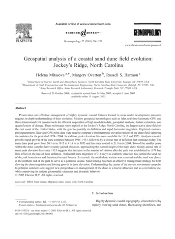
H. Mitasova et al. / Geomorphology 72 (2005) 204–221changes in land cover, represents a significant management challenge. Modern mapping technologies such aslidar and real-time kinematic GPS (RTK-GPS) offer anew approach to short-term monitoring of this dynamicenvironment with unprecedented spatial and temporaldetail. Advanced three-dimensional Geographic Information System (GIS) provides a means for efficientintegration of these new type of measurements withdata from more traditional sources, such as digitizedmaps and photogrammetric surveys. Methods developed for topographic analysis can then be applied tothe digital models of the dunes to quantify the changes inelevation surfaces. This paper presents a multitemporal,high resolution GIS analysis of the Jockey’s Ridge sanddune field on North Carolina (NC) barrier islands withthe aim to gain new insights into geospatial aspects ofthe complex coastal topography and provide valuableinformation for its management.2. The Jockey’s Ridge sand dune fieldJockey’s Ridge, the largest active sand dune fieldon the east coast of the United States, is located within205a 162-hectare state park on the NC Outer Banks (Fig.1). According to previous studies (Havholm, 1996;Runyan and Dolan, 2001), this sand dune fieldbelongs to the class of large, active, isolated coastalcrescentic dunes with little vegetation called medanos.The dunes are asymmetrical, with gentle upwind andsteep downwind sides. In a morphodynamic classification, they are transverse dunes, oriented at angles85–1258 to the dominant sand transport direction(Havholm, 1996). The dune field is complex, comprised of four distinct dunes, each exhibiting a specificmorphology and behavior: east dune, leading southdune, the highest main dune, and a west dune (Fig. 2).Annual wind records document the dominance of SWwinds between March and August and NE windsduring fall and winter months. Based on the datacollected at the U.S. Army Corps of Engineers FieldResearch Facility at Duck, NC, located 27 km to thenorth (USACE FRF, 2004), the mean wind speed forthe period 1982–1999 was 6.1 m/s and the mean winddirection was 1688 (SSE). For each month of the year,the 18 yr average of the mean monthly wind speedexceeded 4.5 m/s critical velocity needed to move thesand. In addition, the annual wind rose for 1982–1999Fig. 1. Location of Jockey’s Ridge dune field on the Outer Banks, the North Carolina barrier islands. Photo shows a view of the dune from theNE after rainfall in 2003.
206H. Mitasova et al. / Geomorphology 72 (2005) 204–221Fig. 2. Dune field elevation surface in 2001 showing location of individual dunes (main, south, east and west), their respective peaks (M1, M2,S, E, W), points on the Soundside Road used for accuracy testing, and representative profiles used for assessment of horizontal dune migration(arrows).indicates that stronger winds (7–20 m/s) from thenorth and northeast are more frequent (USACE FRF,2004), resulting in greater sand transport to the southand southwest. This conclusion is also supported bythe sand transport rose for 1980–1991 (see Fig. 1 byHavholm et al., 2004).Established in 1975, Jockey’s Ridge State Parkhosts around 800,000 visitors each year. When thepark was planned, prevailing opinion considered thedune field relatively stable, characterized only by aslow SW movement (State of North Carolina, 1976).However, encroachment of the dunes onto the roadand homes along the southern border of the park hasbeen an ongoing problem that has required continuingmanagement intervention. The study by Judge et al.(2000) compared the dune topography based on the1974 and 1995 contour maps and demonstrated thelong-term trend of southward migration and deflation.Evolution of the dune field over the past 50 years hasbeen accompanied by dramatic changes in land coverin the surrounding areas, where the sand flats andsmall dunes have been replaced by urban development and a dense maritime forest. As a result, theavailable sand supply has been diminished, thus contributing to the loss of elevation of the main dune.The major challenge for the dune management is tomaintain stability of this highly dynamic feature andkeep it within the park boundaries, while preservingits natural properties as a shifting, migrating dunefield. In recent years, sand fencing was installed onFig. 3. Different spatial patterns and densities of elevation data for the main dune: (A) RTK-GPS traverses in 2002 (black) and 2004 (white); (B)Leica Geosystems aeroscan lidar 2001; (C) NASA/USGS/NOAA Airborne Topographic Mapper II lidar 1999; (D) photogrammetric masspoints 1998; (E) photogrammetrically derived digital contours 1995; (F) digitized contours 1974; (G) 1961 nautical chart with elevations basedon 1953 topographic map; (H) 1932 nautical chart with elevations based on 1915 topographic map. Nautical charts were obtained from theImage Archives of the Historical Map and Chart Collection, Office of Coast Survey, National Ocean Service, NOAA ap.asp).
H. Mitasova et al. / Geomorphology 72 (2005) 204–221207
208H. Mitasova et al. / Geomorphology 72 (2005) 204–221the south dune to slow its migration. In December1995, 15 103 m3 of sand was removed from thepark’s southern boundary; and in the winter of 2003,almost 10 times more sand, 125 103 m3, wasremoved and placed on the northwestern side of thedune field to serve as a sand source area. While someimmediate problems were solved, the long-term effectiveness of this approach is not known and continuedmonitoring is needed to quantify the performance ofindividual management actions at various locations.According to the NC Division of Parks and Recreation (Ellis, 1996), understanding how the dunes function and how they have been affected by the land usechange is essential if they are to be maintained as anaturally functioning system.3. MethodsTo assess the dynamic evolution of the Jockey’sRidge dune complex, a GIS database with multitemporal data layers representing topography and its properties (slope, curvature, peaks, etc.) was established.Methodology for integrating elevation data acquiredby different mapping technologies was developed andtopographic analysis was used to extract the characteristic features of the dunes so that their change could bemeasured. Land cover change was estimated based onhistorical maps and aerial photography.3.1. Data acquisitionThe Jockey’s Ridge dune field elevation was surveyed several times over the past 100 years using avariety of mapping technologies:2002, 2004: Real-time kinematic GPS (RTK-GPS)data were obtained by automatically sampling thesurface along a survey path with a selected step (inour case 1–3 m) and 0.10 m vertical and 0.05 mhorizontal accuracy. Because the movement of vehicles on the dune was restricted, performing RTKGPS survey over the entire dune field was notfeasible in the year 2002. Therefore, only linearand point features (dune crests, ridges, and peaks)that could be identified on digital elevation models(DEMs) as well as in the field were measured.Although this data did not provide information forassessment of volume change, it did permit measurement of the horizontal migration and peak elevation change. After obtaining a special permit, the2004 survey was done using an all terrain vehicle(ATV) and, as a result, covers most of the dune,except for slip faces and vegetated areas (Fig. 3A).2001: Lidar survey by the North Carolina Floodplain Mapping Program (2004) was performedusing Leica Geosystems aeroscan with linear scanning pattern and about 1 point per 3-m density (Fig.3B). Multiple returns taken from an altitude of2300 m enabled extraction of bare ground surfacepoints, with the published vertical accuracy in openareas of 0.20 m and horizontal accuracy of 2 m.1999: Lidar survey by USGS/NASA/NOAA wasdone using the Airborne Topographic Mapper II(for technical details see NOAA Coastal ServicesCenter, 2004; Stockdon et al., 2002). Terrain wassampled from an altitude of 700 m using overlapping 200–300 m swaths and elliptic scanningpattern (Fig. 3C). Elevation was measured every 1–3 m with a reported vertical accuracy of 0.15 m inbare areas and a horizontal accuracy of 0.8 m. Onlythe first return points were acquired, representingthe terrain surface that includes the top of thevegetation and buildings.1998: Spot elevations and breakline points (Fig.3D) were derived from 1 : 7200-scale aerial photography. The published vertical accuracy of the datais 0.06 m for spot elevations and the horizontalaccuracy is 0.30 m.1995: Digital elevation data included contours,breaklines, and spot elevations (Fig. 3E) determinedfrom a photogrammetric survey with a 0.76-m vertical accuracy for contours, 0.03-m accuracy for spotelevations, and a horizontal accuracy of 0.4 m.1974: Digital 1.5-m (5-ft) contours (Fig. 3F) wereacquired from a park map derived from a photo-Fig. 4. Topographic parameters derived from the 1 m resolution 2001 DEM: (A) slope (slip faces in red/magenta); (B) profile curvature (convexcrests in red); (C) uphill slope line density (ridges in brown), inset shows contours and individual slope lines merging on a ridge overlayed bygrid cells with slope values used to compute the average windward ridge slope; (D) extracted crests for 1974 (green), 1995 (blue), and 1998(red) draped over the 2001 surface showing horizontal migration of the Jockey’s Ridge dune complex.
H. Mitasova et al. / Geomorphology 72 (2005) 204–221209
210H. Mitasova et al. / Geomorphology 72 (2005) 204–221grammetric survey, with a 0.7-m vertical accuracyfor contours, 0.15-m accuracy for spot elevations,and a horizontal accuracy of 0.4 m.1953: USGS topographic map, Manteo, NC (Fig.3G) included only few spot elevations representingthe dune peaks and a limited set of contours (10and 15 ft) in the Jockey’s Ridge area complyingwith National Map Accuracy Standards for1 : 24,000-scale mapping. Data were derived from1949 aerial photography using photogrammetrictechniques and 1950 plane table surveys. Thesedata were field checked in 1953 before publishingthe map. At the time of the field verification, thesurveyor’s report indicates that the higher elevationcontours derived from the photogrammetric datacould not be verified. Therefore, these contourswere replaced by spot elevations and a note thatthis was an area of shifting sands. The inability toverify the contours after a 4-year period likelyrepresented real change from 1949 to 1953. Unfortunately for this study, these contours were omittedin the final product.1915: U.S. Coast and Geodetic Survey 1 : 40,000scale T sheet (Fig. 3H) included peaks and a limited set of 3.3-m (10-ft) contours. The contourinterval implies a vertical accuracy of F 1.15 m(5 ft). However, the uncertainty in the elevationvalues is increased by the fact that elevations arereferenced to feet above high water. For this paper,we have not tried to convert from this early datumto NAVD88.In addition to the elevation data, a multitemporalseries of historical charts (1879), aerial photographs(1932, 1940, 1972, 1998, 2003), and historical groundbased photographs (1900–1910) were acquired fromvarious sources and, where possible, imported into theGIS database. These products provided insights intothe spatial distribution of vegetative cover and urbandevelopment as it evolved over the past century.Elevation data from 1974, 1995, 1998, 1999, 2001,and 2004 were geo-referenced in the State Plane coordinate system, horizontal datum NAD83, units feet(the 1974 data were converted from NAD27), verticaldatum NAVD88 (1974 and 1995 data were convertedfrom NGVD29, the difference between NAVD88 andNGVD29 in this location is 0.30 m). To use the fullpower of GIS for analysis and visualization, the lidar,RTK-GPS, and digitized elevation data were transformed to high resolution (1-m) grids creating a multitemporal set of the dune field models.3.2. Spline-based spatial approximation for high resolution DEMsThe input elevation data had different point densities, spatial distributions, and accuracy (Fig. 3A–F).To extract the features needed for quantitative assessment of the dune evolution, a common, high-resolution digital representation is required. Spatialapproximation by the Regularized Spline with Tension and Smoothing method (RST; Mitasova andMitas, 1993; Mitasova et al., 1995) was used forcomputing the 1-m resolution grid DEMs from lidarpoint clouds, digitized contours, and RTK-GPS data.This method is known to produce surfaces withminimum artifacts and high accuracy, even in areaswith sparse data (e.g., Mitasova et al., 1996;Hofierka et al., 2002). In our application, this wasimportant for interpolating some of the contour data,RTK-GPS traverses, and vegetated areas with sparsepoints in the 2001 lidar data set. An additionaladvantage of the method is the capability to simultaneously compute topographic parameters (Mitasovaand Hofierka, 1993), thus ensuring consistencybetween the DEM and the derived slope and curvature maps. The method has been implemented inopen source GRASS GIS (Neteler and Mitasova,2004) as a module called s.surf.rst, which wasused in this project. The 1-m resolution providedsufficient detail for representation of importantdune features, such as active crests and slip facesas well as some man-made features (e.g., partiallyburied fences), without the need for manuallydefined breaklines (Mitasova et al., 2004).To assess the consistency and accuracy of theinterpolated DEMs and to identify potential systematic errors or vertical datum inconsistencies, 40 pointswere selected along Soundside Road, a local pavedroad bordering the park on the south that is assumedto be a stable feature (Fig. 2). Elevation differencesbetween the RTK-GPS elevations (with the highestaccuracy among the methods used) and the interpolated DEMs were computed in the test points. Thedifferences were then used to derive the root meansquare difference (RMSD) and mean absolute differ-
H. Mitasova et al. / Geomorphology 72 (2005) 204–221ence (MAD) as measures of internal consistency forthe multitemporal elevation data set. The RMSD/MAD between the RTK-GPS point data and the interpolated DEMs was between 0.02/0.06 m (1999 DEM)and 0.65/0.43 m (1998 DEM).3.3. Topographic analysis and identification of dunefeaturesTopographic analysis was used to extract featuresdefining the location and geometry of individual211dunes. These features– peaks, slip faces, active crests,windward side ridges, and active dune areas– areessential for measuring the dune migration and understanding its evolution. Slope and profile curvature(Fig. 4A,B), needed for extraction of slip faces anddune crests (Fig. 4D), were computed simultaneouslywith the interpolation of the DEMs using the first- andsecond-order partial derivatives of the RST functionand principles of differential geometry (Mitasova andHofierka, 1993). Previous application of this approachto lidar data demonstrated that suitable selection of theFig. 5. Jockey’s Ridge main dune peak: (A) noise or people captured near the top of the dune in 1999 lidar data; (B) peak migration 1953–2004(1974: dark surface, 2001: light surface); (C) change in elevation 1915–2004.
212H. Mitasova et al. / Geomorphology 72 (2005) 204–221RST parameters (tension and smoothing) is essentialfor extraction of the topographic parameters at thelevel of detail matching the size of the dune features(Mitasova et al., 2004).3.3.1. PeaksAlthough dune peaks can be relatively easy toidentify as the points with the highest local elevation,this task was far from trivial at Jockey’s Ridge andrequired careful analysis of data. In addition to thecommon issues related to the use of different verticaldatums, low curvature of the dune ridge made thepeaks difficult to identify in the field during the 2002and 2004 RTK-GPS surveys. Moreover, the 1999lidar data included points that probably capturedpeople on the top of the dune, increasing the maximum measured elevation more than 1 m above thedune surface (Fig. 5A). These points had to beremoved before determining the 1999 main peakelevation.3.3.2. Active crests and slip facesBased on three-dimensional visual analysis of thedune model with profile curvature draped over theelevation surface as a color map (Fig. 4B), profilecurvature N 0.008 m 1 (convexity) proved to be agood indicator of dune crests. Slopes N308 (close tothe angle of repose for sand) were used to identify theslip faces (Fig. 4A). For the 1999 first-return lidardata, the slopes had to be combined with land cover toexclude the steep slopes caused by vegetation andbuildings.3.3.3. Dune ridgesIn general, ridges can be identified using plan (tangential) curvature; however, this approach is not verysuitable for the dunes with smooth windward sides andlow values of curvature. Therefore, an alternativeapproach based on the density of slope lines (lines inthe direction of surface gradient, perpendicular to contours) generated uphill from each grid cell was used(Mitasova et al., 1996). This approach is an inverseversion of the flow accumulation algorithm commonlyused for extraction of streams (e.g., Tarboton, 1997),where slope lines are traced downhill from each celland cells with slope line density (flow accumulation)exceeding a given threshold define the stream network.To extract ridges, slope lines were computed using aD-infinite (vector-grid) algorithm (Mitasova et al.,1996) to avoid artificial patterns produced by thestandard D-8 methods on smooth surfaces typical fordunes. Dune ridges were then extracted as grid cellsthat had the number of slope lines passing throughthem (slope line accumulation) N 600 (Fig. 4C). Theaverage slope of the windward side of the dunes wasthen computed by manually defining representativewindward profiles along these ridges, extractingslope values along the profiles from the slope mapsusing map algebra, and computing the average valuefor each dune (Fig. 4C insert).3.3.4. Active dune subregionVisual analysis of contours, generated from theDEMs at 0.3 m interval and displayed along withelevation, slope and land cover maps, was used 2004(B)Fig. 6. Evolution of the dune field: (A) horizontal migration of individual dunes given as cumulative distance measured between the dune crestsalong representative profiles (see Fig. 2) and (B) dune volume and area change for the active dune subregion defined by elevation z N 6 m.
H. Mitasova et al. / Geomorphology 72 (2005) 204–221213Fig. 7. Overlay of active dune surfaces (subregions without vegetation where elevation z N 6 m), demonstrating similar patterns of southwardmigration between (A) 1974– 1995 and (B) 1995– 2001. Higher of the two surfaces is visible and migration of the main peak is represented byarrow. Inserts show changes in slip faces: (A) reversal in the slip face direction from east in 1974 to west in 1995 on the lower ridge of the maindune and (B) evolution of a new slip face binsideQ the main dune in 1999.
214H. Mitasova et al. / Geomorphology 72 (2005) 204–221identify a threshold elevation that defines the activedune subregion. Topography below this thresholdflattens and includes only small, mostly stable vegetated features. Elevation surface above the thresholdhas typical dune geometry and bare sand. For allDEMs (1974 – 2001) this threshold elevation wasfound to be 6 m. For the 1999 DEM, the elevationthreshold had to be combined with land cover derivedfrom the 1998 aerial photography to eliminate treesand buildings. Map algebra was then used to compute the active dune DEMs as surfaces with elevation z N 6 m.3.3.5. Quantification of the dune changeJockey’s Ridge, as a complex dune field, has spatially and temporally variable migration, growth, anddeflation rates (Fig. 6A). To quantify its evolution, anapproach based on topographic analysis of elevationsurfaces that involves extraction of dune features andmeasurement of the change in their location was used(Fisher et al., 2005). High resolution DEMs and GIStools make such analysis feasible and effective.To assess the dune field evolution, the multitemporal set of DEMs was first analyzed visually usingthree-dimensional models of overlayed surfaces andFig. 8. Long-term and short-term elevation differences revealing continuing sand loss on the northern, windward side of the dunes and gainmostly on the southern side of the dunes along the slip faces: (A) 1974–1995; (B) 1995–1998; (C) 1999–2001; and (D) cross-section of the maindune showing dune flattening between 1999 and 2001 (profile is colored by the bottom surface).
H. Mitasova et al. / Geomorphology 72 (2005) 204–221interactive cutting planes (Fig. 7 and 8D; Neteler andMitasova, 2004). Map algebra, spatial query, andrelated standard GIS tools were then used to computethe maps and summary values for the following measures quantifying the dune change:(i) change in the elevation and location of the dunepeaks,(ii) horizontal migration of the dune field,(iii) spatial pattern of elevation change,(iv) evolution of active dune volume and area, and(v) change in the windward ridge slope.Exact measurement of the horizontal dune migration was challenging because of the complex, changing morphology of the dune field. Representativeprofiles were defined perpendicular to the slip facesin the locations where the crests could be clearlyidentified for each DEM in the multitemporal dataset (Fig. 2). These profiles were used to trace themovement of individual dunes within this field andto identify potential differences in the migrationrates. The horizontal migration of a dune was measured as a distance between the two consecutivelocations of the active dune crest along these profiles. To quantify the rate of lateral dune migration,the shortest distance between two consecutive locations of windward side ridges, as defined by slopeline densities (Fig. 4C), was measured. Change inthe shape and size of crests and ridges contributed touncertainty in the measurements; therefore, each distance was measured six times and an average valuewas computed. The standard deviations of theseaverages did not exceed 3 m.4. ResultsVisual comparison of high resolution elevationsurfaces representing the dune in 1974, 1995, 1998,1999, 2001, and 2004 confirms the prevailing southern migration of the entire dune field (Fig. 7) accompanied by dune deflation. Apparently, the overalldirection of dune migration to the SW is not dictatedby the long-term mean wind orientation (winds fromthe SE). Rather, as shown by the sand transportrose presented by Havholm et al. (2004), the higherfrequency of stronger winds from NE (see also215USACE FRF, 2004) lead to the prevailing SW direction of the potential sand transport. In addition, shortterm changes may show up in any particular survey ifthe morphology captured was strongly influenced by arecent storm. Two of the data sets, 1998 and 1999,were post-storm surveys. The June 1998 flight captured the impact of a late season northeaster thatoccurred in early May. In addition, the 1999 lidarflight was planned as a response to Hurricane Dennis.Hurricane Dennis moved north along the NC coast on31 August 1999, remained until 2 September, loststrength to tropical storm status, and then came ashoreon 5 September. The lidar flight was conducted lessthan a week later on 9–10 September. Data from theUSACE FRF (2004) showed that the maximumonshore winds were 24 m/s from the NE on 31August. Following this peak, the wind speed averagedabout 15 m/s from the NW to NE through 4 September and then rotated and resumed the dominant direction (SE). While it was the intent of this study tocapture long-term changes, the measurements do,however, record topographic modifications resultingfrom essentially instantaneous short-term events. Analysis of specific dune features, described in the following sections, provides more detailed informationabout dune evolution while also revealing the underlying complexity of its behavior.4.1. MorphologyVisual analysis of the three-dimensional dunemodels and spatial patterns of crests and slip facesrevealed a complex dynamic morphology within thedune field (Figs. 4, 7 and 8). While several featurespoint to the prevailing crescentic transverse dunes, adetailed analysis shows additional types of dunesevolving over time. The leading tip of the eastdune has evolved into a low, fast-moving parabolicdune. The main dune has a complex, dynamic morphology, including a high ridge, with a distinctsouth-oriented slip face and an extended low ridgewith a west-oriented slip face. This slip face hasflipped its direction from east to west between1974 and 1995 (Fig. 7A insert), leading to changein the direction of its migration. The high section ofthe main dune often develops an east-facing slip face(Fig. 4A). The leading south dune was an eggshaped mound in 1975 that was transformed into a
216H. Mitasova et al. / Geomorphology 72 (2005) 204–221parabolic dune (Fig. 7A). The west dune has evolvedinto a characteristic crescentic dune shape withcurved slip faces.4.2. Peak changeThe dune peak evolution was tracked using historical maps dating from 1915 when the first topographicmapping that included measurement of dune elevationwas performed. According to this survey, the maximum elevation in the area was 20.1 m (66 ft, Fig.3H), which is less than the current elevation of 21.9 m(71.8 ft) and less than one-half of the Jockey’s Ridgemaximum elevation, recorded on the 1953 topographic map as 42.1 m (138 ft, Fig. 3G). The 1915and 1953 maps indicate that the main dune wasgrowing rapidly at a rate of about 0.6 m/yr between1915 and 1953. Sometime after 1953, the main dunepeak (M1 in Fig. 2 and Table 1) started to loseelevation (Fig. 5C) at an average rate of 0.36 m/yr.The peak on the lower, western ridge of the main dune(M2 in Fig. 2 and Table 1) was 23.5m high in 1974,and after losing elevation between 1974 and 1998,this peak started to grow again and is now almost ashigh as the main peak (21.8m). East dune peak (E inFig. 2 and Table 1), was losing elevation at a rate 0.12m/yr between 1953 and 1998, but its elevationincreased 2.3 m between 1998 and 2004 at an annualrate of 0.38 m/yr. Elevation of the west dune peak(W), held steady at around 20 m.The horizontal main peak migration followed thesoutheast direction between 1953 and 1995, with aneastward turn between 1995 and 1998, then continuing in south-southeast direction in the following years,with the exception of 2001–2002 time interval, whenTable 1Evolution of the dune peaks’ elevationa: the highest main dune peakM1, peak on the west ridge of main dune M2 (see Fig. 2), east dunepeak E and west dune peak WPeak1915 1950 1974 1995 1998 1999 2001 2002 2004
morphology and behavior: east dune, leading south dune, the highest main dune, and a west dune (Fig. 2). Annual wind records document the dominance of SW winds between March and August and NE winds during fall and winter months. Based on the data collected at the U.S. Army Corps of Engineers Field Research Facility at Duck, NC, located 27 km to the