Transcription
KONINKL. NEDERL. AKADEMIE VAN WETENSCHAPPEN - AMSTERDAMReprinted from Proceedings, Series A, 75, No. 5 and Indag. Math., 34, No. 5, 1972MATHEMATICSLAMBDA CALCULUS NOTATION WITH NAMELESS DUMMIES,A TOOL FOR AUTOMATIC FORMULA MANIPULATION,WITH APPLICATION TO THE CHURCH-ROSSER THEOREMN. G. DE BRUIJN(Comrnunicatod at tho mooting of Juno 24, 1972)I n ordinary lambda calculus the occurrences of a bound variable are maderecognizable by the use of one and the same (otherwise irrelevan ) name a t alloccurrences. This convention is known to cause considerable trouble in cases ofsubstitution. I n the present paper a different notational system is developed, whereoccurrences of variables are indicated by integers giving the "distance" to thebinding L instead of a name attached to that A. The system is claimed to be efficientfor automatic formula manipulation as well as for metalingual discrission. As anexample the most essential part of a proof of the Church-Rosser theorem is presentedin this namefree calculus.For what lambda calculus is about, we refer to [I], [3] or [4], althoughno specific knowledge will be required for the reading of the present paper.Manipulations in the lambda calculus are often troublesome because ofthe need for re-naming bound variables. For example, if a free vzriable inan expesssion has to be replaced by a second expression, the danger arisesthat some free variable of the second expression bears the srtrne name asa bound variable in the first one, with the effect that binding is introducedwhere i t is not intended. Another case of re-naming arises if we want toestablish the equivalence of two expressions in those situations where theonly difference lies in the names of the bound variables (i.e. when theequivalence is so-called a-equivalence).I n particular in machine-ma.nipulated lambda calculus t h i s re namingactivity involves a great deal of labour, both in machine time as inprogramming effort. It seems to be worth-whila to try to get rid of there-naming, or, rather, to get rid of names altogether.Consider the following three criteria for a good notation:(i) easy to write and easy to read for the human reader;(ii) easy to handle in metalingual discussion;(iii) easy for the computer and for the computer programmer.The system we sha.11 develop here is claimed to be good for (ii) and
good for (iii). It is not claimed to be very good for (i); this means thatfor computer work we shall want automatic translation from one of theusual systems to our present system a t the input stage, and backwardsa t the output stage.An example showing that our method is adequate for (ii) can be foundin sections 10-12, which present the kernel of a proof for the ChurchRosser theorem. This proof is essentially the one that was given in [I],where it was attributed to P. Martin-Lof (1971). Later private informationby Mr. H. P. Barendregt disclosed that the idea is due to W. W. Tait.For a survey of proofs of the Church-Rosser theorem see [ l ] p. 16-17.An elaborate treatment of the theorem can also be found in [4].What is said about lambda calculus in this paper ritn be applied directlyto other kinds of dummy-binding in mathematics. For example, if wehave an cxprewion like thc product 17,,,f(k, rtr), we can write i t asn ( p , q, Akj(k, m ) ) . For any new quantifier we wish to use (like 17 here)we have to take a particular symbol that is treated as an element of thealphabet of constants (see section 3).Application to AUTOMATH is explained in section 13.If we want to denote a string of symbols by a single ("metalingual")symbol, we have to be very careful, in particular if this procedure isrepeated, e.g. if we form mixed strings of lingual and metalingual symbols,represent these by a new symbol, etc.We shall use parentheses ( ) for this purpose. If rP denotes a string,then @ is not the string itself. For the string itself we shall use (@). Weshall say that @ denotes the string and that (@) is the string. Let usconsider some examples, where the basic lingual symbols are all Latinletters as well as the hyphen. (These examples will show the use of ( )in nested form, and therefore show that the simple device of using Greekletters on the metalingual level is definitely insufficient.) We shall use thesymbol e for reversing the order of a string. That is, e(pqra) denotes arqp,whence e(pqra)) arqp. Now let @ denote the word phi, and let 2 denotethe word sigma. Then (@)(Z) is the word phisigma, i@.tr)-(Z) phi-sigma,(e((Z))) amgis, and (e(ihpamgis)) sigmaphi (Z)(@).The ( )'s of this section are not to be confused with the similar symbolswe use in Backus' normal form of a syntax (e.g. in section 5).I n typescript and in handwriting it is convenient to underline a formulainstead of putting i t in ( )'s. I n print, however, underlining, and inparticular multi-level underlining, is awkward.
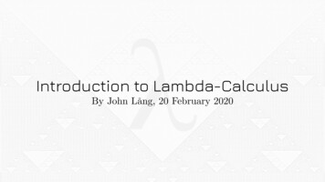
3. N AME-CARRYING EXPRESSIONSWe explain the kind of lambda calculus expressions which we want toturn into riamefree expressions. We have a set of "constants" (a, b, c, f, g, .)and a set of "variables" (s, t , u, v, w, x, .). And there is the symbol Athat can have any variable as a suffix. Moreover we admit application,of which the following is the interpretation. If @ denotes a function, anda value of the variable, thenis the value of the functiona t ( r ) . We shall use a different notation instead: we add a symbol Ato the list of con stunt, , and we write A((@), (r))instead of (@)((I').This puts it on a ptbr with another kind of exprwsion we are going toadmit, viz. things like f ( , ,), where f is any constant. I n the interpretationsthe latter kind of expression can be very close to what wc have just calledapplication, but that does not bother us a t the moment.We shall not go into a formal definition of the syntax; the followingexample (that accidentally does not contain the symbol A a t all) will beclear enough. We take the expressionr4.(@)((r))GETTINGRIDOF THE NAMES OF VARLABLESI n order t)o facilitate the discussion, we represent the expression as aplanar tree which is easier to read than (3.1) itself.If in (3.1) we change the names of the bound variables, e.g. x, t, u, sinto p, u, s, x, we get an expression that is what is usudly called orequivalent to (3.1):&Oub(p, u, f ( W s , u, z), Axw)), w, y).We shall take the simplistic point of view that or-equivalent expressionsare the same. Formula (3.1) contains bound variables rc, d, u, s and freevariables z , w, y. We shall keep a list of letters from which the freevariables are to be taken. Let that list be, in this order, z, v, w, y ; wedraw the points Az, Av, A,, A, under the tree.The rariables in the tree (fig. 1) are encircled (unless they occur as asuffix of 1).For every encircled letter we evaluate two integers which are indicatedin the fignre, viz. the reference depth and the level. The reference depthof an encircled variable a t a certain spot, x say, is the number of A's weencounter when running down until we meet As (this Ax is counted as oneof the encountersd A's). It is agreed that the ILy,A, A,, A, (which do notbelong to the tree idself) can also be encountered on our way down, e.g.if we run down to 3, we encounter A, A, A,, 1,.The level of an encircled variable st a certain spot counts the totalnumber of A's we encounter when running down the tree until we get tothe root (if the root is a A, like A, here, this one is also included in thecount; the loose A, A,, A,, il, are not counted this time.
Let us now eraso the variables and the integers indicating the levels;we keep the reference depth. No information is lost: the erascd lettersand numbers can be easily reconstructed. If we are not interested in thenames of the bound variables (and honestly we should not be) we canerase the suffix in A%, At, Au, AS. I n those eases where we are interestedin the names of the free variables we have to keep the ordered list 2, v,w, yin order to be able to reconstruct our expression. Note that a point ofthe tree refers t o a free variable if and only if the reference depth exceedsthe level.'Fig. 1 .1 7I h u s the information contained in our name-carryiug expression canb(: presented as(4.1 )w w , 1 , fw,2 , 7 a w , 3 , )with the free variable list z, v, w, y. This expression is called namefree.Note thatl (3.1) can be represented difft-rently if we take a differentfree vuriable list. Any sequence of distinct variables may serve as a freevariable list provided i t contains z, to, y in any order. Conversely, everynamefree expression can be decoded into a name-carrying one if we providea free variable list that is long enough. This determines the name-carryingexpression up to name-changing of the hound variables.
Instead of providing a finite free variable list we can take an infiniteone (with the effect that we need not bother whether the list is longenough). The reference depths refer to a count in the reference list fromright to loft, corresponding to the fact that A's are written in front of theformula thcy act, on. Therefore, such infinite free variable lists have tobc written as ., xs, x2, x1 instead of the usual left-to-right notation ofan infinite sequence.5.THE S Y N T A X FOR NAMEFREE EXPRESSIONSWe present the syntax in Backus' normal form:(NF expression string) : : (NF expression)l(NF expression string),(NF expression)(NF expression) :: (constant) j(constant)((NF expression string))/(positive integer) lL(NP expression)In the next sections we shall use, in an informal way, the notions"level" of an integer in an N F expression, in the sense of section 4. (The"reference depth" of an integer is, of course, the integer itself).6.SX BSTITUTIQNMTcshall definc the effect of a substitution of a sequence of NF expressions into a single N F expression denoted by 9.Whet we intend to describe is the foflow-ing. Let ., &, 22, Z; denotethe sequence (in right-to-left notation). (In practice only finitely many&'s m' rc!evant; whence we need not always give the full infinite sequence). We attach a free variable list ., x xz,, x to Q, and one and thes Irne free variable list . , ya, yz, yl to every .Xi.That determines namec wrying expressions to be denoted by Q* and &*. Now replace any free.x, in (Q*) by the corresponding (&*). Thus we get an expression, to bedenoted hywith possible free v a r i a b k . ., y3, ya, yl. With respect t othis freo variable list ., ya,yz, yl thisriwresponds to the NF expression, (. . X 3 ) ,(&j, ( a ) ; (Q)) wre shall define presently. The definition willbe recnrsivr with respect to the structure of (Q); Q may denote eithera n NP' expression qtring or nn NP expression. W e follow the syntacticclassiiwation of seciion 5 .r*r*
386(iii) If S) (y)((91)) (where y denotes a constant and 91 a n NFexpression string) then(4., (23), (22), ( 2 1 ); ( 9 ) ) ) y ) ( W . . -,G 3 ) , (Z2 ¶(Zl? ; (Ql)D)(iv) If ( 9 ) is the positive integer k: then(S(., (&), (E2 ,( W ; (Q))) (.ck). A(r)then(s(., (z3),(z2:2),(z;);( a ) ) ) n ( S (., (A,), ( n 2 A ,,1; (r ) ( v ) If ( 9 )(64where At denotes(a(., 4, 3, 2 ; ( 2 6 ) ) ) .(6.2)Note that ( A a ) is obtained from (&) by adding 1 to every integerin (2f) that refers to a free variable.It will be convenient to use the separate notation t h ( ( 2 ) )in order toabbreviateS( ., h 3, h 2 , & I ; (L')).It means adding h (which is a positive integer) to every integer ( Z )that refers to a free variable. The special case T I ( ( & ) )occurs in (6.2).With the aid of this notation we can give a more global description ofhow (B( ., (.Z3),( Z Z ) ,(21); ( 9 ) ) )is obtained: start from L?,and in eachcase where an integer 1 in (0)exceeds its level E, we replace that t by d(&-l))).I11 antnrnntic formula manipulation it may be a good strategy to refrainfrom evaluating such tl((Z))'s,but just to store them as pairs E , ( X ) ,and go into (full or partial) evaluation only if necessary. The followingformulas may come in handy:8.BE rr,RIDIJCTIOXIf we i i n w an applicstioual expression A((@),( r ) ) (cf. section 3), thentht. interpretatiol is that (@) is a function,a value of the variable(r)
(r))(r).(r)in that function, and A ( ( @ ) ,is intended to represent the value ofthe function (@) a t the pointIf (di) happens to have the formA(Q), then the function value can actually be evaluated. Roughly speaking,it comes down to substitutingin (52) for all occurrences of the boundvariable corresponding to the A in front of (9).A precise definition in terms of NF expressions is easy to give: If 52and r denote NF expressions, thcn A(&@, ( r ) )is an NF expressionto which beta reduction can be applied. The effect of thc bcta rcductionis the NF expressionThe usual beta reduction for name carrying expressions is obtained if weuse one and the same free variable list for all four expressions A(52),A(A(Q),and (8.1). n,(r))ETA REDUCTIONIn terms of name-carrying expressions, 7-reduction means the following.If 2' denotes a name-carrying expression that does not contain the variablem, then A5()7)(x) (or in our notation & A ( ( Z ) ,x ) ) has the same mathematical interpretation as (2') itself. The transfer from Ax(Z)(x)to (Z)is called 7-reduction. We shall define i t for NF expressions:For any NF expression ( A ) we define as 7-reduction the transition of9.(9.1)AA((t,((A))), 1 ) into ( A ) .If we transform both expressions of ( 9 . 1 ) into name-carrying expressionsby means of one and the same free variable list, the transition ( 9 . 1 ) becomes the 7-reduction for name-carrying expressions.MULTIPLEBETA REDUCTIONI n section 8 we considered beta reduction of an NF expression. It wasrednction of the full expression and not the beta reduction of a sube x p r s s i o(local beta reduction) which we shall consider presently. Inordcr to be able to indicate where the p-reduction has to be carried out,we introduce R set of constants (applicational symbols) to be used instead(dt h e single symbol A. By this same device we get the possibility ofmultiple local beta reduction : we indicate a subset of t,he set of applicationalsymbols and we carry out beta reduction for all symbols of that subset.Let, r/' be a subset of the set of constants. An NF expression ( 2 )iscalled U-correct if every element of U that occurs in ( Z ) is always followedby a string in parentheses with the form (;E(52), (r)).I n other words,each orcurrence of each element of U is ready for local beta reduction.To be more precise, we indicate how the syntax of section 5 is to be changedin ordcr to get the syntax of the U-correct NF expressions. We have toreplace the entries10.
(constant) I(constant)((NF expression string))by(constant not in U)l(constant not in U)((NF expression string))/(constant in U)(I(NF expression), (NF expression))a,nd, moreover, we have to write "U-correct NF" instead of "NF" throughout.The following theorem is intuitively clear, and easily proved formallywith the aid of the recursive definition of substitution (section 6).THEOREM10.1. If Q, &, 2-,, . denote U-correct expressions, thenon the set of U-correct N F expressWe shall now define the operatorions recursively :(i) If (Z) is a single constant or a positivc integer, then(ii) If (Z) (y)((&),(iii) If (Z) l(Zl)., (Zk)), where (y) is a constant not in U, thenthenS'ieedless to say, the effect of /3 u on an expression string (Zi), ., (Zk)is to be defined by (@u((Z;))), ., (Pu((&))).11.THEOREMSONMULTIPLE BETA REDUCTIONTHEOIEEM11 .I. If ( 9 , (&), (&),.are U-correct, thenF s o o For:easier reading we shall drop the blgns j and ( throughoutt61s proof.The proof has to be read twice. The first time we deal with the proof ofin the case that the Zi are integers. (This case is intuitively clear, butit tt ireslittle extra trouble to derive it formally.) I n the second readingt!rc result8 of the first reading c m be used.W e apply indiwtion with respect to the structure of 9 , using the definitionof mbstitt tionILR giwn i n m:tion 0. (Note that in the first reading thc
induction hypothesis is used only for cases belonging to the first reading.)The cases (i), (ii), (iv) of section 6 are very simple, and so is case (iii)if the constant y is not in U. We concentrate on the two remaining cases,viz. S L U and SL y(RA, r) with y E I / .If SL 21' we apply (v) of section 6 twice :whcre At is given by (6.2), and At* S( ., 4,3 , 2; BuZ;).By section 10 (iii) and by the induction hypothesis, the right-handside of (11.2) equalsIn the first reading of the proof the & and At are integers, whencepUZt 2 6 , and therefore At* At B u n . So the right-hand sides of ( 1 1.3)and (11.4) are equal, hence the left-hand sides of (ll.2j and (11.3) are equal.I n the second reading of the proof we may use the theorem for the casethat the & are integers; henceand the right-hand sides of (11.2) and (11.3) are equal.The second case we have to deal with, is SL y(lA,with y E U. Wehave to showr)The right-hand side equals, by section 10 (iv)By the formulas on composite substitution (section 7) this isThe left-hand side of (11.5) equals, according to 6 (iii),By 6 (v) we haveS(., 2 2 , .Z& AA) A @where@ S (., A,, A,, 1; A ) , Ag S( ., 3, 2; Xi).Applying 10 (iv) we can write for (11.7)133 the induction hypothesis we have
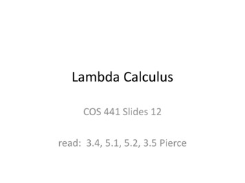
m d so we C L L apply the formula for composite substitution (section 7)to (11.8); i t becomeswherenl s(., 2, 1, BUS( ., z2,21;r ) ;i) pus(., z2,z;; r )n i , S ( ., 2, 1, pus(., ZZ,Z;; r ) B;u A t ) (i 1, 2 , .).We have t o show that ( 11.9) equals ( 11.6). By the induction hypothesis wehave fi S ( . ., B U Z Z , B u Z l ; Bur),so it remains to show that Ui 1 @u&( i l2,, .).I n the first reading of the proof the Z; are positive integers. Thereforethe A( are integers 1 ; it follows that BuAi At 1, whence I7f rlr - 1 z; puz;.I n the second reading of the proof we may use the result of the firstreading :puAl ,9us( ., 3, 2 ; Z t ) S (., 3, 2;j3&),-and thc formula forZ7i 1now results in (cf. section 7)THEOREM11.2. Let U and V be subsets of the set of constants, andlet ( Z ) be both U-correct and V-correct. Then ( / ? u ( ( Z ) ) ) is V-correct, Bv( Z ) is U-correct and (Bu( B ( ( 2 ) ) ) ) ) B v ( ( B u ( ) ) ) .PROOF:Again we omit the ('s and )'s. The V-correctness of @ u Z iseasily proved by recursion: use the definition of j 3 of section 10. I n10 ( i v ) we have to use Theorem 10.1.By the same recursion we shall prove Bu/ vZ /?V#?UZ.The only casewhcrc the induction step is non-trivial is the case Z y(.%Q,withy E U u V . If y E U we have by 10 ( i v )r)By Theorem 1 1.1 this equalsIf J C , 7'EV we find by 10 ( i i ) , 10 (iii)and by 10 (iv) this equals ( 11.10). So y E Ti' u V impIies that PvBuZequals ( 11.10). On behalf of the induction hypothesis ( 11.10) is symmetric,whcnce P v B o S - / ? v Z .THE CHURCH-ROSSERTHEOREM FOR BETA REDUCTIONWe consider an NETexpression Z with a single constant A that can beused fur @-reduction.We label all A's in 2 so that they become all different.12.
Next we take a subset U of the labelled A's, we apply BU and then removethe labels. This gives an N F expression Z. We say that 2' is a multiplereduction of Z', and we write Z 2, 2''. If U has only one element, andif that element ha,s just one occurrence in Z, the reduction is called single,and we write Z 2, 27.If 21 and Zi satisfy either Z; , & or ZZ 8 Zl, we write 21 &.The Church-Rosser theorem for beta reduction says : If Z;2 2. Z;tthen there are Al, ., Ak and Ill, ., I l h with-Z; 8A1 8. 8Ak, 2%2 8 n; 2, . 28nh,-NNAk Jl;r.This can now be proved as follows. From theorem 11.2 we easily obtain :if Zl 2, Zz, Z; , ,273 then there is a Z4 with Z 2 m .&, 2 3 2, Z4.Moreover it can be shown: If Z , A then there is a, sequence(Actually, if every element of U occurs a t most once in the U-correctexpression 2; then we can arrange the elements of U as ul, ., u, insuch a way thatBru,,, Bru,) z BuZ).The Church-Rosser theorem now follows by a trivial reduction argument.The above proof can be easily adapted to lambda calculus with expressions as types (see section 13).NOTATIONIN AUTOMATHThe mathematical language AUTOMATH (see [2]) has lambda calculuswith types, and these types are again expressions. That is, instead of 2,we have things that can be visualized as ;l,, ,(Q),) where d, and Qdenote name-carrying expressions. We may think of x to be a variableof the type (@). It is clear that we do not want x to have any bindinginfluence on (@). I n order to achieve this, we create a new lingual constantT (just like we added A to our set of constants in section 3), and we write13.instead of A,,(,)(Q). Now (13.1) can be transformed into a namefreeexpression just like any other name-carrying expression.The actual notation in AUTOMATH is different. Instead of (13.1)AUTOMATH uses [x, (@)](Q), and for the application A((@), ( r ) )AUTOMATH uses ((T)}(@).14. ALGORITHMS.An algorithm for turning an N F expression into a name-carrying one,can be described on the basis of the recursive definition of substitutionin ection6. Let (Q) be an N F expression. Take a free variable list., 53, Q,XI consisting of distinct letters which do not belong to our
alphabet of constants. Now idd thesc xi to that ;tl -,hitluet,and evaluateThis is a namefree expression; if we proclaim the xi's to be variablesagain, i t becomes an intermediate expression where the free variableshave names but the bound variables are nameless. i f we want to havenames for the bound variables too, we have t o modify S slightly. We takean infinite store of letters yl, yz, . (different from the X S ' S and difiSerentfrom the constants), and we take a modified form of (6.1). Any time weget t o apply (6.1) we take a fresh y (i.e. one that has not been used before)and we replace the right-hand side of (6.1) byIt is not very hard either to give algorithms that transform name-carryingexpressions into namefree ones. This can be done if a free variable list isgiven (and then it has to be checked, during the execution of the algorithm,whether this list is adequate), but we can also write an algorithm thatproduces a free variable list itself. For the case of the first-mentionedpossibility we give a brief description of the crucial steps. Let ., 23, XZ,21be a free variable list, and let (52) be the name-carrying expression wewant to transfer into the namefree expression (Q*). If (52) equals oneof the x's, then (Q*) is an integer, viz. the index of that x. If (52) is avariable, but not one of the x's, the answer is "free variable list waswrong". If (Q) il,(r)then we transform ( r )into the nameless expressionby means of the free variable list23, XZ,21, yl and we have(Q*) l ( r * )The. other cases (the cases (i) (0) (GI), ,/522), (ii) (52) a constant, (iii) (52) (8)((521))) are very easy.(r*).,Technological University,Department of Mathematics,Eindhoven, h7etherlands.REFERENCES1. BARENDREUT,H. P., Some extensional models for cornbinatory logics and Acalculi. Doctorrtl Thesis, Utrecht 1971.2. BRUIJN,N. G. DE, The mathematical language AUTOMATIP, its usage, andsome of its extensions, Symposium on Automatic, Dornonstration(Vorsailles Docember 19681, Lecture Notes in Mathematics, Vol. 125,Springer-Verlag, 29-6 1 ( 1970).3. CHURCH,A., The Calculi of Lambda Conversion. Annals of Math. Studies, vol. 6 ,Princeton University Press, 1941.4. CURRY,Ti. B. and R. FEYS,Combinatory Logic. North-Holland PublishingCompany, Amsterdam 1958.
LAMBDA CALCULUS NOTATION WITH NAMELESS DUMMIES, A TOOL FOR AUTOMATIC FORMULA MANIPULATION, WITH APPLICATION TO THE CHURCH-ROSSER THEOREM N. G. DE BRUIJN (Comrnunicatod at tho mooting of Juno 24, 1972) In ordinary lambda calculus the occurrences of a bound variable are made recognizable by the use of one and the same (otherwise irrelevan ) name .