Transcription
NBER WORKING PAPER SERIESEMPIRICS OF STRATEGIC INTERDEPENDENCE:THE CASE OF THE RACIAL TIPPING POINTWilliam EasterlyWorking Paper 15069http://www.nber.org/papers/w15069NATIONAL BUREAU OF ECONOMIC RESEARCH1050 Massachusetts AvenueCambridge, MA 02138June 2009 I am grateful for comments received from David Romer, two anonymous referees, Ingrid GouldEllen, participants in the CEPR Conference on Macroeconomics and Geography in Modena Italy,those in the NBER Summer Institute on Macroeconomics and Inequality, and those in a seminar atUC-Berkeley. The views expressed herein are those of the author(s) and do not necessarily reflectthe views of the National Bureau of Economic Research.NBER working papers are circulated for discussion and comment purposes. They have not been peerreviewed or been subject to the review by the NBER Board of Directors that accompanies officialNBER publications. 2009 by William Easterly. All rights reserved. Short sections of text, not to exceed two paragraphs,may be quoted without explicit permission provided that full credit, including notice, is given tothe source.
Empirics of Strategic Interdependence: The Case of the Racial Tipping PointWilliam EasterlyNBER Working Paper No. 15069June 2009JEL No. D85,O10,R0,Z13ABSTRACTThe Schelling model of a “tipping point” in racial segregation, in which whites flee a neighborhoodonce a threshold of nonwhites is reached, is a canonical model of strategic interdependence. The ideaof “tipping” explaining segregation is widely accepted in the academic literature and popular media.I use census tract data for metropolitan areas of the US from 1970 to 2000 to test the predictions ofthe Schelling model and find that this particular model of strategic interaction largely fails the tests.There is more “white flight” out of neighborhoods with a high initial share of whites than out of moreracially mixed neighborhoodsWilliam EasterlyNew York UniversityDepartment of Economics19 W. 4th Street, 6th floorNew York NY 10012and NBERwilliam.easterly@nyu.edu
21. IntroductionModels of strategic interaction are common in the economic growth literature, aswell as in many other fields. For example, in human capital spillover models of economicgrowth, your incentive to acquire human capital depends on the human capital of others.If spillovers take place within neighborhoods, then strategic interactions affectneighborhood formation, human capital of different ethnic groups, and overall inequality(Borjas 1993, 1996, Benabou 1993, 1996, Durlauf 2002, 1999, 1996). These modelsoften feature multiple equilibria and sensitivity to initial conditions. Although the theoryis well developed, there has been only limited empirical testing of strategic interactionsand sensitivity to initial conditions.2One of the most famous models of strategic interaction in economics is ThomasSchelling’s (1971) elegant model of racial segregation (see its coverage in Dixit andNalebuff 1991, for example). He shows how only a modest preference of whites to livenext to other whites could result in nearly complete residential segregation, because ofthe instability of intermediate points where one agent’s residential location depends onthe actions of other agents in the neighborhood. In this model, even a relatively smallfraction of nonwhites could cause the neighborhood to “tip” from completely white tocompletely nonwhite. The fraction at which this happens is called the “tipping point.”Segregation outcomes might seem to reflect segregationist preferences by whites,but in the Schelling model the degree of segregation exceeds what all but a smallminority of the white population desires. If there are differences in average human capital2Borjas 1993, 1996 shows empirically that outcomes for individuals are affected by “neighborhoodcapital” and “ethnic capital”, but does not test for sensitivity to initial conditions in neighborhoodformation.
3between whites and blacks, and there are spillovers within neighborhoods, thenresidential segregation has important implications for black-white income differences.Card and Rothstein (2007) find that the black-white test score gap is higher in moresegregated cities. Hence, Schelling’s model is potentially one of the important buildingblocks in understanding inequality (Durlauf 2002 cites it in this context).The tipping view of neighborhood change had been around long beforeSchelling’s piece. Schelling (1971) says he was inspired by articles from the 1950s,where the tipping process was described as universal, as was the instability of mixedneighborhoods. Once a neighborhood had begun to change from white to black, there wasrarely a reversal. The process was very nonlinear. An article in 1960 defined it thus:Although the movement of whites out of the area may proceed at varying rates of speed, a“tipping point” is soon reached which sets off a wholesale flight of whites. It is not toolong before the community becomes predominantly Negro.3The idea of the “tipping point” is very much alive today both in academicliterature and in popular folklore. Sociologists Douglas Massey and Nancy Denton (1993)describe how a white “majority still feel uncomfortable in any neighborhood that containsmore than a few black residents; and as the percentage of blacks rises, the number ofwhites who say they would refuse to enter or would try to move out increases sharply.”Ellen (2000) sums up the current conventional wisdom similarly: “racially integratedneighborhoods cannot stay that way for long because as soon as the black population ina neighborhood has reached some “tipping” point, whites move away in droves.”4 Arecent paper by Card, Mas, and Rothstein (2008) (discussed further below) reaffirms the3Oscar Cohen quoted in Wolf (1963).Ellen (2000) does not share this conventional wisdom, arguing for a more nuanced view of “whiteavoidance” of integrated neighborhoods for reasons unrelated to race. She argues that racially mixedneighborhoods in 1990 were more common and more stable than the conventional wisdom would have it.4
4story that, in their words, “once the minority share exceeds the tipping point, theneighborhood transitions rapidly to a very high minority share.”A large social science literature studies racial segregation. However, the Schellingmodel has undergone surprisingly little large-scale empirical testing on residentialneighborhoods. There has been extensive empirical testing of the determinants ofsegregation using survey methods to ascertain people’s preferences for segregation, ortesting small samples of neighborhoods or school districts, or testing cross-citydeterminants of segregation, some of which address the Schelling hypothesis (with mixedresults).5 In a Galllup survey in 1997, 25 percent of whites said they would move ifblacks came in “great numbers” into their neighborhood (which was a large decreasefrom 73 percent in a similar survey in 1966). This seems to indicate an increasedtolerance for racial integration among whites over time. However, the researchers whoreport this survey result (Schuman et al.1997) still believe in the tipping point model:“the upward trend does not seem to match reality if compared with the exodus of whitefamilies that often occurs when large numbers of black families move into a previouslywhite neighborhood” (pp. 152-153).The Multi-City Study of Urban Inequality (O’Connor, Tilly and Bobo 2001)conducted a more nuanced survey in Atlanta, Boston, Detroit, and Los Angeles. Theyshowed whites five different cards indicating neighborhood composition ranging from5See Clark (1991), Galster (1988), Clark (1988), Massey and Gross (1991), Wilson (1985), Farley et al.(1994), Giles (1978), Farley and Frey (1994), Hwang and Murdock (1998), Giles et al. (1975), Wolf(1963), and Schwab and Marsh (1980). Denton and Massey (1991) analyze transition matrices for a largesample of metropolitan census tracts from 1970 to 1980, but do not test the nonlinear dynamic equationimplied by the Schelling model. Massey and Denton (1993) extensively discuss neighborhood transitionswith census tract data, but do not test the tipping point hypothesis. Crowder (2000) does do a regression ofindividual level mobility on neighborhood nonwhite share that shows a highly nonlinear relationship aspredicted by the tipping point model, but his setup does not lend itself to explicitly testing for a tippingpoint. Clotfelder (2001) finds the growth of white enrollment in schools declines almost linearly over mostof the range of exposure to nonwhites in school districts.
5all-white to majority black and asked them if they would “feel comfortable” in suchneighborhoods or would be “willing to move in” to such a neighborhood. The affirmativeresponse by whites falls fairly sharply as the black share rises, which would be moreconsistent with the tipping point hypothesis (for example, only 30 percent of whiteswould be willing to move into a neighborhood with an 53 percent black majority, withslightly more “feeling comfortable.”)6Despite the popularity of the tipping model, there has been little in the way offull-scale test of the tipping point hypothesis with nationwide data on Americanmetropolitan neighborhoods.7 The major exception is Card, Mas, and Rothstein 2008,who use the same data as this paper (the data will be described next) and a regressiondiscontinuity design to test for racial tipping points based on the local stability ofintermediate points of minority share. They did find evidence of tipping at relatively lowlevels of minority share. Their methodology has the important advantage that they canderive from the data a different tipping point for each metropolitan area, allowing fordifferent sensitivity to minority share across metropolitan areas. This paper (whose firstversion preceded Card et al.) differs from Card et al by estimating the global dynamics oftipping based on initial racial composition. To accommodate the highly non-linearprediction of the Schelling model, I estimate the change in white share as a function of afourth-order polynomial of initial white share. I first assume that the tipping point is thesame in all neighborhoods, and then will allow tipping points to vary parametrically withother neighborhood characteristics. These two different methodologies allow for testing6Charles 2001, pp. 233-237Aaronson (2001) and Ellen (2000) also run regressions for neighborhood dynamics using census tract datafrom 1970 to 1990, but they do not explicitly test the tipping point hypothesis. Both have indirect resultsthat tend to indicate stability of neighborhood racial composition, which would be in line with this paper’sconclusions.7
6of different predictions of the tipping model – the model has predictions both for localinstability and for global dynamics. The Card et al. approach economizes on assumptionsabout parametric forms, however it does so at the cost of being only a test of localinstability. Local instability is necessary but not sufficient for confirmation of the tippingmodel. The advantage of this paper’s approach is that it tests also the global dynamicspredictions that are also required to confirm the tipping story.These tests have become feasible thanks to the availability of a new database fromthe Urban Institute and a firm called Geolytics.com, which matches census tractinformation from the U.S. censuses for 1970, 1980, 1990, and 2000. This is called theNeighborhood Change Data Base (NCDB). The database covers metropolitan areas; itdoes not include rural areas.This database confirms that American neighborhoods continue to be highlysegregated in the year 2000, despite some decrease in segregation and despite years ofrhetoric and legal action in favor of integration. Nonwhites made up 28 percent of thesample population in the NCDB in 2000. Blacks make up 14 percent of the samplepopulation. If each neighborhood were a random draw of whites and nonwhites, with theprobability of drawing a nonwhite .28, the odds against a neighborhood nonwhite shareof less than 10 percent would be astronomical. Yet 35 percent of all census tracts hadnonwhite shares less than 10 percent. Similarly, the probability that a nonwhite wouldlive in a neighborhood where the nonwhite share exceeds 50 percent would be extremelylow if the population were distributed randomly. Yet the median black lived in aneighborhood that was 52 percent black. The Tauber dissimilarity index, a widely usedindicator of segregation, was .53 in the year 2000 for America as a whole (the index
7ranges from 0 if nonwhites are evenly distributed across neighborhoods to 1 if whites andnonwhites are completely segregated). The index can be interpreted as the fraction ofeither whites or nonwhites that would have to move to achieve even distributions of racialgroups across neighborhoods.8 I do not attempt in this paper to cover the rich literature onthe historical and modern mechanisms determining racial segregation; I am just doing atest of one particular model of segregation.9Of great relevance for the tipping point hypothesis, changes in neighborhoodsfrom majority white to majority nonwhite are common in the dataset. Of the 41,321urban census tracts in the NCDB that have data for both 1970 and 2000, 3965neighborhoods had a drop in white share of .5 or greater from 1970 to 2000. Thus nearly10 percent of the neighborhoods in the sample changed drastically from majority white tomajority nonwhite over these 30 years. A weaker definition of tipping, the change fromany white majority in 1970 to a nonwhite majority in 2000, reveals 14 percent of theneighborhoods tipped during this 30 year period.This paper uses this database to conduct tests of some of the predictions of theSchelling “tipping point” model. It will ask the fundamental question of whether the highdegree of segregation observed in American neighborhoods is a consequence of thedynamic instability of intermediate points due to strategic interdependence, with onlyweak preferences for living next to your own racial group.8See the discussion by Cutler, Glaeser, and Vigdor 1999 of different measures of racial segregation. Theyalso present evidence that segregation declined from 1970 to 1990.9See Massey and Denton (1993), Ellen (2000), and Meyer (2000) for a richer treatment of the complexitiesof residential segregation.
82. Schelling’s modelSchelling’s model is simple and elegant. Suppose that whites’ preferences forneighborhood segregation between whites and blacks can be summarized as follows:each white individual j has an individual-specific preference to live in a neighborhoodthat has at least wj percent of whites. If white individual j finds himself in a neighborhoodcontaining less than wj percent of whites, then he will exit the neighborhood. As long asthe neighborhood contains more than wj percent of whites, then individual j will stay inthe neighborhood. Whites have diverse preferences for racial segregation ranging fromintegrationist to segregationist, which can be summarized by a cumulative densityfunction increasing from zero to one over wj from zero to one. Thus, the cumulativedensity function gives us the percent of whites that have an wj less than or equal to w.The CDF therefore shows the percent of whites that will live in a neighborhood that is wpercent white – it is all those who have an wj less than or equal to w.To relate the CDF to the whites who desire to live in the neighborhood as afraction of the neighborhood population, one set of assumptions consistent with hismodel is that whites have a right of first refusal on the homes in any neighborhood – soall the homes are offered to a representative sample of whites, F(w) of whom accept. Theremainder of homes are then occupied by non-whites. Hence F(w) also gives the ratio ofwhites desiring to live in the neighborhood to the total neighborhood population.Note that Schelling’s basic model assumes the outcome is entirely driven bywhites’ preferences. This assumption is debatable (and perhaps even offensive), but itreflects the traditional view of neighborhood segregation as mainly driven by whites’behavior. It could be justified by saying that whites have stronger preferences about
9getting their preferred racial composition than nonwhites, and hence will pay more to livein their preferred neighborhood (note that the basic Schelling model does not have anyrole for housing prices). Schelling actually did a version of the model that alsoincorporated nonwhites’ preferences for neighborhood composition, but it has not caughton like the original model and it did not dramatically change the predictions of the model.The point where the cumulative density function crosses the 45 degree line iswhere the fraction of whites willing to live in a neighborhood that is w percent white is infact equal to w:(1) w F(w)This is an equilibrium outcome for racial composition of the neighborhood; there will bemore than one such point since CDFs satisfy F(0) 0 and F(1) 1. The tipping point storyonly makes sense if (1) also holds for an intermediate point between 0 and 1.The dynamics of the white share can be specified by giving the change in whiteshare as the distance between the CDF and the 45 degree line.(2) Δw F(w) – wThis is the equation that will actually be estimated in the empirical section, using a veryflexible fourth order polynomial.Now suppose also that (3) holds.(3) F’(w) 1 evaluated at a point strictly less than 1 and strictly greater than 0 where(1) holds.If (3) holds, then one of the points where (1) holds is an unstable equilibrium. In otherwords, (1) and (3) define a tipping point. Any w above this point will spiral upwards
10towards greater segregation of mostly white neighborhoods, and any w below it willshow white flight and more segregated black neighborhoods.10Suppose for illustration that the CDF is of the normal distribution with mean μand variance σ2, F(w;μ,σ2), For example, assuming just for illustration that μ .75 andσ .1, Figure 1 shows the corresponding cumulative density function.10(3) could hold at w 1, in which case w 1 is a tipping point. However, this is not what Schelling had inmind, since he discusses a shift from a stable neighborhood above the tipping point.
11Figure 1: The cumulative normal distribution for racial preferences10.9normal(u .75,se .1)0.845 degree lineCumulative normal and 45 degree are of whites0.81
12The CDF is highly nonlinear, with flat segments at either end but climbing steeplyin the middle. This reflects the characteristics of the normal distribution, with flat tails butsteep increases in the number of individuals contained in the middle. The actual fractionof whites who live in the neighborhood is given by the 45 degree line.Note that the tipping point is a higher fraction of whites w than the mean of thenormal distribution of white preferences. For example, in the figure the equilibrium pointis .86, while the mean of the normal distribution was .75. Any mean of the normaldistribution greater than .5 cannot be an equilibrium or a tipping point, because only .5 ofwhites are willing to live in the neighborhood with the mean of the normal distributionfor fraction of whites. The tipping point always lies above the mean in this case.If there is a disturbance to a neighborhood in the vicinity of the tipping point suchthat a few whites leave the neighborhood or a few nonwhites enter and the white sharedrops below equilibrium, then the fraction of whites willing to live in the neighborhoodfalls below the actual share. There is a further decrease in white share, and yet a furtherwhite exodus. This process does not stop until the neighborhood becomes completelynonwhite – a white share of 0 is a stable equilibrium. The neighborhood has “tipped”from being majority white to completely nonwhite.Conversely, any deviation of the white share above the equilibrium will lead to afraction of whites willing to live in the neighborhood that is greater than the actual share.This will cause the white share to increase. A new equilibrium is not reached until thecumulative density function intersects the 45 degree line from above. In the diagram, thishappens at a white share of about .992. Hence, the remarkable outcome of Schelling’s
13model is that the long run equilibrium is for neighborhoods to be either entirely nonwhiteor 99.2 percent white, despite the preferences of the median white for a mixedneighborhood that is 75 percent white and 25 percent nonwhite.Although the tipping point idea is linked historically to racial scare-mongeringabout the “threat” of nonwhites moving into the neighborhood, Schelling’s contributionactually gives quite a different perspective on racial segregation. The point of Schelling’smodel was that the strategic interdependence of weak preferences for living next topeople of the same race could lead to an outcome of almost total segregation. Suppose asmall increase in nonwhites around the tipping point of a neighborhood with high whiteshare directly causes only the most racist white to exit the neighborhood. However, thedeparture of the most racist white causes a further decrease in white share, which nowleaves the second-most racist white uncomfortable with fewer white neighbors, and healso leaves. (I do not mean to imply that people have to move sequentially and gradually,this is just for illustration.) This in turn leaves the third most racist white discomfited, andhe leaves. So things keep unraveling until even relatively integrationist whites wind upexiting, until the whole neighborhood tips over, all because of an initial small increase innonwhites that only directly bothered the most racist white. This contrasts with the viewthat segregation reflects whites having a very strong preference for having whiteneighbors. Hence a test of Schelling’s model is a test of whether residential segregationsimply reflects the interaction of what could be weak average preferences for same-raceneighbors. The alternative is that segregation is something more fundamental driven byother factors.
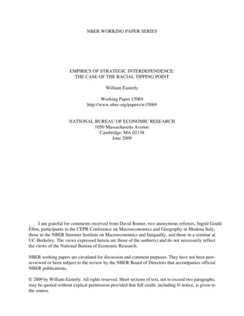
14In figure 1, the fall in white share is dramatic below the tipping point, reflectingthe rapid movement through the fat part of the normal distribution of the wj. This accordswell with the classic story of tipping as a rapid exodus of whites out of the neighborhoodonce tipping begins. However, we have no evidence that the distribution is normal or anyother distribution, and the prediction of very rapid exodus comes out of somedistributions and not others. A CDF could be much closer to the 45 degree line below thetipping point and still satisfy conditions (1) through (3).In general, some CDFs do not fit the classic “tipping point” narrative, eventhough they have tipping points. For example, think of a simple distribution where thereare only three discrete groups of whites, each containing one-third of the whitepopulation. The first has a wj of 0.3, the second of 0.6, and the last of 0.9. This wouldgenerate the CDF shown in Figure 2. This CDF features no less than 4 stable equilibria(zero white, minority white, majority white, and all white) and 3 tipping points. Tippingis a relatively more modest affair between these stable equilibria, and each group has aneighborhood close to their preferences, in contrast to the massive reversal and differencebetween preferences and outcomes in the normal distribution tipping story. The classictipping story relies on a distribution of whites who are fairly similar to one another andthus vulnerable to chain reactions; more heterogeneity of preferences leads to more stableoutcomes closer to preferences. The advantage of this paper’s methodology inestimating the entire distribution (2) is that it allows for the “classic” tipping point storyto be compared to two alternatives: (a) there are no tipping points, and (b) there aretipping points but the CDF does not fit the “classic” global tipping story. The Card et al.2008 approach, in contrast, can only rule out (a), not (b).
15Figure 2: Tipping Points with 3 heterogeneous groups of whites1Tipping points0.90.80.70.6cumx0.50.40.30.20.1Stable equilibria000.10.20.30.40.50.60.70.80.91One last set of considerations when taking the model to the data is considering theoverall outcome. When whites exit a neighborhood that is tipping nonwhite, where dothey go? Obviously, they would go to a neighborhood with a higher white share, and sothey become part of those neighborhoods that are tipping towards greater white share.However, note that the Schelling model is not a general equilibrium model. Thereis no adding up constraint to enforce that the population-weighted average ofneighborhoods’ white share be equal to the system-wide share of whites in thepopulation. Because all neighborhoods are subject to random shocks of varying intensity,the Schelling model does not place any restrictions on how many of the neighborhoodswill be in the segregated nonwhite equilibrium or in the higher segregated whiteequilibrium. Hence, one cannot reject a particular estimated tipping point on the groundsthat it is inconsistent with overall white share.
16However, other possible estimated outcomes of equation (2) could be inconsistentwith overall population structure. If (2) shows a globally stable intermediate equilibriumwhich is different than the overall white share, then that does violate adding upconstraints. Similarly, if the estimated equation (2) implies a dynamic structure in whichall neighborhoods converge to all-white (or all-nonwhite), then that would also obviouslyviolate the adding up constraint. Such violations would call into question that what hasbeen estimated is in fact a global dynamic structure, as opposed to a relationship betweeninitial white share and predicted changes in white share (which could be one timechanges) that are explained by other stories besides the Schelling model.3. The dataThe database used in this analysis was originally called the Underclass Database(UDB). It was put together for 1970, 1980, and 1990 by the Urban Institute, a nonpartisanthink tank in Washington DC. Given the interests of the Institute, the data coveredmetropolitan neighborhoods (where “metropolitan” is defined as in the census to includecentral city, inner suburbs, and outer suburbs). The database has been updated to includethe 2000 census by a commercial firm called Geolytics Inc.11 The unit of analysis in thedatabase is the census tract, a division meant to approximate a “neighborhood”, usuallycontaining between 2500 and 8000 people. The tract boundaries are chosen to captureneighbors with similar social characteristics (which means that measures of segregationbased on tract data will tend to exaggerate segregation). Tract boundaries do not crosscounty, metropolitan area, or state boundaries.1211The new database is available on CD-ROM from geolytics.com. The description of the data containedhere is based on the NCDB Data User’s Guide, including Appendix J on tract matching.12Except in New England, some tracts cross metropolitan area boundaries.
17There are several difficult issues surrounding the data construction. Of those tractsthat have data for both 1970 and 2000, two-thirds changed boundaries. Some tracts weremerged into a single tract, and some single tracts were divided into multiple tracts.Unfortunately, in the majority of tract changes, there are boundary changes that are notsimple mergers or divisions of existing tracts. The constructors of the database addressedthis problem in several different ways, depending on what data was available for differentcensus years. They used geographic information software (GIS) to overlay 2000 tractboundaries on earlier tract boundaries. They then used 1990 block data to estimate theproportion of the old tracts in various racial categories that went into the new tract, andthen recalculated the 1990 tract data using the 2000 tract boundaries.Block data located spatially were not available for 1970 and 1980. The 1980 tractswere matched to the 1990 tracts and 1970 tracts matched to 1980 tracts using CensusBureau information on tract correspondence based only on spatial changes in tractboundaries. Hence, the 1970 and 1980 tract matching to 1990 and 2000 is less accuratethan the tract matching between 1990 and 2000.The database includes an indicator of which tracts changed boundaries. The use ofthe full sample could be justified if we think any errors introduced by boundary changesare random, i.e. uncorrelated with the right hand side variables in my regressions below.However, I will run a robustness check of my results by running them on the sub-samplewhich did not change boundaries between 1970 and 2000.Some 2000 tract boundaries include areas that were not covered at all by 1970data. As long as the covered area is a random sample of the whole tract, with the errorterm uncorrelated with the 1970 white share, the use of the full sample could still be
18justified. Nevertheless, I will run another robustness check by omitting these observationsfrom the sample.Census data has the commonly known problem that it undercounts the populationbecause some people are harder to reach for enumeration. Of concern for our exercise,the undercount is thought to be proportionally greater for nonwhite populations. Theundercount percentage has been falling over time. I do not have any solution to thisproblem, but hope that it is of small enough magnitude not to distort the results. In 1990,the Census estimated the overall undercount as 2 percent, down from 5 percent in 1950.The undercount for blacks was estimated at 5.7 percent in 1990, an increase from 4.5percent in 1980.13Table 1 shows the variable definitions and summary statistics. The sample is allavailable data in the NCDB, which as I noted is mainly for metropolitan census tracts(Map 1 shows the coverage of NCDB fo
discontinuity design to test for racial tipping points based on the local stability of intermediate points of minority share. They did find evidence of tipping at relatively low levels of minority share. Their methodology has the important advantage that they can derive from the data a different tipping point for each metropolitan area .