Transcription
Graph Representation LearningWilliam L. HamiltonMcGill University2020Pre-publication draft of a book to be published byMorgan & Claypool publishers.Unedited version released with permission.All relevant copyrights held by the author andpublisher extend to this pre-publication draft.Citation: William L. Hamilton. (2020). Graph Representation Learning.Synthesis Lectures on Artificial Intelligence and Machine Learning, Vol. 14,No. 3 , Pages 1-159.
iiAbstractGraph-structured data is ubiquitous throughout the natural and social sciences,from telecommunication networks to quantum chemistry. Building relational inductivebiases into deep learning architectures is crucial if we want systems that can learn,reason, and generalize from this kind of data. Recent years have seen a surge in researchon graph representation learning, including techniques for deep graph embeddings,generalizations of convolutional neural networks to graph-structured data, and neuralmessage-passing approaches inspired by belief propagation. These advances in graphrepresentation learning have led to new state-of-the-art results in numerous domains,including chemical synthesis, 3D-vision, recommender systems, question answering,and social network analysis.The goal of this book is to provide a synthesis and overview of graph representationlearning. We begin with a discussion of the goals of graph representation learning, aswell as key methodological foundations in graph theory and network analysis. Following this, we introduce and review methods for learning node embeddings, includingrandom-walk based methods and applications to knowledge graphs. We then providea technical synthesis and introduction to the highly successful graph neural network(GNN) formalism, which has become a dominant and fast-growing paradigm for deeplearning with graph data. The book concludes with a synthesis of recent advancementsin deep generative models for graphs—a nascent, but quickly growing subset of graphrepresentation learning.
ContentsPrefaceviAcknowledgmentsvii1 Introduction1.1 What is a graph? . . . . . . . . . . . . . . . . . . . . .1.1.1 Multi-relational Graphs . . . . . . . . . . . . .1.1.2 Feature Information . . . . . . . . . . . . . . .1.2 Machine learning on graphs . . . . . . . . . . . . . . .1.2.1 Node classification . . . . . . . . . . . . . . . .1.2.2 Relation prediction . . . . . . . . . . . . . . . .1.2.3 Clustering and community detection . . . . . .1.2.4 Graph classification, regression, and clustering.1223446772 Background and Traditional Approaches2.1 Graph Statistics and Kernel Methods . . . . .2.1.1 Node-level statistics and features . . .2.1.2 Graph-level features and graph kernels2.2 Neighborhood Overlap Detection . . . . . . .2.2.1 Local overlap measures . . . . . . . .2.2.2 Global overlap measures . . . . . . . .2.3 Graph Laplacians and Spectral Methods . . .2.3.1 Graph Laplacians . . . . . . . . . . . .2.3.2 Graph Cuts and Clustering . . . . . .2.3.3 Generalized spectral clustering . . . .2.4 Towards Learned Representations . . . . . . .9910131616182121232627INode Embeddings.283 Neighborhood Reconstruction Methods293.1 An Encoder-Decoder Perspective . . . . . . . . . . . . . . . . . . 303.1.1 The Encoder . . . . . . . . . . . . . . . . . . . . . . . . . 303.1.2 The Decoder . . . . . . . . . . . . . . . . . . . . . . . . . 31iii
3.23.33.43.1.3 Optimizing an Encoder-Decoder Model . . . . .3.1.4 Overview of the Encoder-Decoder Approach . . .Factorization-based approaches . . . . . . . . . . . . . .Random walk embeddings . . . . . . . . . . . . . . . . .3.3.1 Random walk methods and matrix factorizationLimitations of Shallow Embeddings . . . . . . . . . . . .4 Multi-relational Data and Knowledge Graphs4.1 Reconstructing multi-relational data . . . . . .4.2 Loss functions . . . . . . . . . . . . . . . . . . .4.3 Multi-relational decoders . . . . . . . . . . . . .4.3.1 Representational abilities . . . . . . . .II.313232343636.3839404244Graph Neural Networks465 The Graph Neural Network Model5.1 Neural Message Passing . . . . . . . . . . . . . . . .5.1.1 Overview of the Message Passing Framework5.1.2 Motivations and Intuitions . . . . . . . . . .5.1.3 The Basic GNN . . . . . . . . . . . . . . . . .5.1.4 Message Passing with Self-loops . . . . . . . .5.2 Generalized Neighborhood Aggregation . . . . . . .5.2.1 Neighborhood Normalization . . . . . . . . .5.2.2 Set Aggregators . . . . . . . . . . . . . . . . .5.2.3 Neighborhood Attention . . . . . . . . . . . .5.3 Generalized Update Methods . . . . . . . . . . . . .5.3.1 Concatenation and Skip-Connections . . . . .5.3.2 Gated Updates . . . . . . . . . . . . . . . . .5.3.3 Jumping Knowledge Connections . . . . . . .5.4 Edge Features and Multi-relational GNNs . . . . . .5.4.1 Relational Graph Neural Networks . . . . . .5.4.2 Attention and Feature Concatenation . . . .5.5 Graph Pooling . . . . . . . . . . . . . . . . . . . . .5.6 Generalized Message Passing . . . . . . . . . . . . .474848505152525354565859616162626364666 Graph Neural Networks in Practice6.1 Applications and Loss Functions . . . .6.1.1 GNNs for Node Classification . .6.1.2 GNNs for Graph Classification .6.1.3 GNNs for Relation Prediction . .6.1.4 Pre-training GNNs . . . . . . . .6.2 Efficiency Concerns and Node Sampling6.2.1 Graph-level Implementations . .6.2.2 Subsampling and Mini-Batching6.3 Parameter Sharing and Regularization .68686970707172727273iv.
v7 Theoretical Motivations7.1 GNNs and Graph Convolutions . . . . . . . . . . . . . . . .7.1.1 Convolutions and the Fourier Transform . . . . . . .7.1.2 From Time Signals to Graph Signals . . . . . . . . .7.1.3 Spectral Graph Convolutions . . . . . . . . . . . . .7.1.4 Convolution-Inspired GNNs . . . . . . . . . . . . . .7.2 GNNs and Probabilistic Graphical Models . . . . . . . . . .7.2.1 Hilbert Space Embeddings of Distributions . . . . .7.2.2 Graphs as Graphical Models . . . . . . . . . . . . .7.2.3 Embedding mean-field inference . . . . . . . . . . . .7.2.4 GNNs and PGMs More Generally . . . . . . . . . .7.3 GNNs and Graph Isomorphism . . . . . . . . . . . . . . . .7.3.1 Graph Isomorphism . . . . . . . . . . . . . . . . . .7.3.2 Graph Isomorphism and Representational Capacity .7.3.3 The Weisfieler-Lehman Algorithm . . . . . . . . . .7.3.4 GNNs and the WL Algorithm . . . . . . . . . . . . .7.3.5 Beyond the WL Algorithm . . . . . . . . . . . . . .III.Generative Graph Models8 Traditional Graph Generation Approaches8.1 Overview of Traditional Approaches . . . .8.2 Erdös-Rényi Model . . . . . . . . . . . . . .8.3 Stochastic Block Models . . . . . . . . . . .8.4 Preferential Attachment . . . . . . . . . . .8.5 Traditional Applications . . . . . . . . . . 41051079 Deep Generative Models9.1 Variational Autoencoder Approaches . . . . . .9.1.1 Node-level Latents . . . . . . . . . . . .9.1.2 Graph-level Latents . . . . . . . . . . .9.2 Adversarial Approaches . . . . . . . . . . . . .9.3 Autoregressive Methods . . . . . . . . . . . . .9.3.1 Modeling Edge Dependencies . . . . . .9.3.2 Recurrent Models for Graph Generation9.4 Evaluating Graph Generation . . . . . . . . . .9.5 Molecule Generation . . . . . . . . . . . . . . ography125
PrefaceThe field of graph representation learning has grown at an incredible–and sometimes unwieldy—pace over the past seven years. I first encountered this area asa graduate student in 2013, during the time when many researchers began investigating deep learning methods for “embedding” graph-structured data. Inthe years since 2013, the field of graph representation learning has witnesseda truly impressive rise and expansion—from the development of the standardgraph neural network paradigm to the nascent work on deep generative models of graph-structured data. The field has transformed from a small subsetof researchers working on a relatively niche topic to one of the fastest growingsub-areas of deep learning.However, as the field as grown, our understanding of the methods and theories underlying graph representation learning has also stretched backwardsthrough time. We can now view the popular “node embedding” methods aswell-understood extensions of classic work on dimensionality reduction. Wenow have an understanding and appreciation for how graph neural networksevolved—somewhat independently—from historically rich lines of work on spectral graph theory, harmonic analysis, variational inference, and the theory ofgraph isomorphism. This book is my attempt to synthesize and summarizethese methodological threads in a practical way. My hope is to introduce thereader to the current practice of the field, while also connecting this practice tobroader lines of historical research in machine learning and beyond.Intended audience This book is intended for a graduate-level researcherin machine learning or an advanced undergraduate student. The discussionsof graph-structured data and graph properties are relatively self-contained.However, the book does assume a background in machine learning and afamiliarity with modern deep learning methods (e.g., convolutional and recurrent neural networks). Generally, the book assumes a level of machinelearning and deep learning knowledge that one would obtain from a textbook such as Goodfellow et al. [2016]’s Deep Learning Book.William L. HamiltonAugust 2020vi
AcknowledgmentsOver the past several years, I have had the good fortune to work with manyoutstanding collaborators on topics related to graph representation learning—many of whom have made seminal contributions to this nascent field. I amdeeply indebted to all these collaborators and friends: my colleagues at Stanford,McGill, University of Toronto, and elsewhere; my graduate students at McGill—who taught me more than anyone else the value of pedagogical writing; and myPhD advisors—Dan Jurafsky and Jure Leskovec—who encouraged and seededthis path for my research.I also owe a great debt of gratitude to the students of my winter 2020 graduate seminar at McGill University. These students were the early “beta testers”of this material, and this book would not exist without their feedback and encouragement. In a similar vein, the exceptionally detailed feedback provided byPetar Veličković, as well as comments by Mariá C. V. Nascimento, Jian Tang,Àlex Ferrer Campo, Seyed Mohammad Sadegh Mahdavi, Yawei Li, XiaofengChen, and Gabriele Corso were invaluable during revisions of the manuscript.No book is written in a vacuum. This book is the culmination of years ofcollaborations with many outstanding colleagues—not to mention months ofsupport from my wife and partner, Amy. It is safe to say that this book couldnot have been written without their support. Though, of course, any errors aremine alone.William L. HamiltonAugust 2020vii
viiiACKNOWLEDGMENTS
Chapter 1IntroductionGraphs are a ubiquitous data structure and a universal language for describingcomplex systems. In the most general view, a graph is simply a collection ofobjects (i.e., nodes), along with a set of interactions (i.e., edges) between pairs ofthese objects. For example, to encode a social network as a graph we might usenodes to represent individuals and use edges to represent that two individualsare friends (Figure 1.1). In the biological domain we could use the nodes in agraph to represent proteins, and use the edges to represent various biologicalinteractions, such as kinetic interactions between 21328314252220269Figure 1.1: The famous Zachary Karate Club Network represents the friendshiprelationships between members of a karate club studied by Wayne W. Zacharyfrom 1970 to 1972. An edge connects two individuals if they socialized outsideof the club. During Zachary’s study, the club split into two factions—centeredaround nodes 0 and 33—and Zachary was able to correctly predict which nodeswould fall into each faction based on the graph structure [Zachary, 1977].The power of the graph formalism lies both in its focus on relationshipsbetween points (rather than the properties of individual points), as well as inits generality. The same graph formalism can be used to represent social networks, interactions between drugs and proteins, the interactions between atoms1
2CHAPTER 1. INTRODUCTIONin a molecule, or the connections between terminals in a telecommunicationsnetwork—to name just a few examples.Graphs do more than just provide an elegant theoretical framework, however. They offer a mathematical foundation that we can build upon to analyze,understand, and learn from real-world complex systems. In the last twenty-fiveyears, there has been a dramatic increase in the quantity and quality of graphstructured data that is available to researchers. With the advent of large-scalesocial networking platforms, massive scientific initiatives to model the interactome, food webs, databases of molecule graph structures, and billions of interconnected web-enabled devices, there is no shortage of meaningful graph datafor researchers to analyze. The challenge is unlocking the potential of this data.This book is about how we can use machine learning to tackle this challenge.Of course, machine learning is not the only possible way to analyze graph data.1However, given the ever-increasing scale and complexity of the graph datasetsthat we seek to analyze, it is clear that machine learning will play an importantrole in advancing our ability to model, analyze, and understand graph data.1.1What is a graph?Before we discuss machine learning on graphs, it is necessary to give a bit moreformal description of what exactly we mean by “graph data”. Formally, a graphG (V, E) is defined by a set of nodes V and a set of edges E between thesenodes. We denote an edge going from node u V to node v V as (u, v) E.In many cases we will be concerned only with simple graphs, where there is atmost one edge between each pair of nodes, no edges between a node and itself,and where the edges are all undirected, i.e., (u, v) E (v, u) E.A convenient way to represent graphs is through an adjacency matrix A R V V . To represent a graph with an adjacency matrix, we order the nodesin the graph so that every node indexes a particular row and column in theadjacency matrix. We can then represent the presence of edges as entries in thismatrix: A[u, v] 1 if (u, v) E and A[u, v] 0 otherwise. If the graph containsonly undirected edges then A will be a symmetric matrix, but if the graph isdirected (i.e., edge direction matters) then A will not necessarily be symmetric.Some graphs can also have weighted edges, where the entries in the adjacencymatrix are arbitrary real-values rather than {0, 1}. For instance, a weightededge in a protein-protein interaction graph might indicated the strength of theassociation between two proteins.1.1.1Multi-relational GraphsBeyond the distinction between undirected, directed and weighted edges, wewill also consider graphs that have different types of edges. For instance, ingraphs representing drug-drug interactions, we might want different edges to1 The field of network analysis independent of machine learning is the subject of entiretextbooks and will not be covered in detail here [Newman, 2018].
1.1. WHAT IS A GRAPH?3correspond to different side effects that can occur when you take a pair of drugsat the same time. In these cases we can extend the edge notation to includean edge or relation type τ , e.g., (u, τ, v) E, and we can define one adjacencymatrix Aτ per edge type. We call such graphs multi-relational, and the entiregraph can be summarized by an adjacency tensor A R V R V , where R isthe set of relations. Two important subsets of multi-relational graphs are oftenknown as heterogeneous and multiplex graphs.Heterogeneous graphs In heterogeneous graphs, nodes are also imbuedwith types, meaning that we can partition the set of nodes into disjoint setsV V1 V2 . Vk where Vi Vj , i 6 j. Edges in heterogeneousgraphs generally satisfy constraints according to the node types, most commonly the constraint that certain edges only connect nodes of certain types,i.e., (u, τi , v) E u Vj , v Vk . For example, in a heterogeneous biomedical graph, there might be one type of node representing proteins, one typeof representing drugs, and one type representing diseases. Edges representing“treatments” would only occur between drug nodes and disease nodes. Similarly, edges representing “polypharmacy side-effects” would only occur betweentwo drug nodes. Multipartite graphs are a well-known special case of heterogeneous graphs, where edges can only connect nodes that have different types,i.e., (u, τi , v) E u Vj , v Vk j 6 k.Multiplex graphs In multiplex graphs we assume that the graph can bedecomposed in a set of k layers. Every node is assumed to belong to everylayer, and each layer corresponds to a unique relation, representing the intralayer edge type for that layer. We also assume that inter-layer edges types canexist, which connect the same node across layers. Multiplex graphs are bestunderstood via examples. For instance, in a multiplex transportation network,each node might represent a city and each layer might represent a different modeof transportation (e.g., air travel or train travel). Intra-layer edges would thenrepresent cities that are connected by different modes of transportation, whileinter-layer edges represent the possibility of switching modes of transportationwithin a particular city.1.1.2Feature InformationLastly, in many cases we also have attribute or feature information associatedwith a graph (e.g., a profile picture associated with a user in a social network).Most often these are node-level attributes that we represent using a real-valuedmatrix X R V m , where we assume that the ordering of the nodes is consistent with the ordering in the adjacency matrix. In heterogeneous graphs wegenerally assume that each different type of node has its own distinct type ofattributes. In rare cases we will also consider graphs that have real-valued edgefeatures in addition to discrete edge types, and in some cases we even associatereal-valued features with entire graphs.
4CHAPTER 1. INTRODUCTIONGraph or network? We use the term “graph” in this book, but you willsee many other resources use the term “network” to describe the same kindof data. In some places, we will use both terms (e.g., for social or biologicalnetworks). So which term is correct? In many ways, this terminologicaldifference is a historical and cultural one: the term “graph” appears tobe more prevalent in machine learning communitya , but “network” hashistorically been popular in the data mining and (unsurprisingly) networkscience communities. We use both terms in this book, but we also makea distinction between the usage of these terms. We use the term graph todescribe the abstract data structure that is the focus of this book, but wewill also often use the term network to describe specific, real-world instantiations of this data structure (e.g., social networks). This terminologicaldistinction is fitting with their current popular usages of these terms. Network analysis is generally concerned with the properties of real-world data,whereas graph theory is concerned with the theoretical properties of themathematical graph abstraction.a Perhaps1.2in some part due to the terminological clash with “neural networks.”Machine learning on graphsMachine learning is inherently a problem-driven discipline. We seek to buildmodels that can learn from data in order to solve particular tasks, and machinelearning models are often categorized according to the type of task they seekto solve: Is it a supervised task, where the goal is to predict a target outputgiven an input datapoint? Is it an unsupervised task, where the goal is to inferpatterns, such as clusters of points, in the data?Machine learning with graphs is no different, but the usual categories ofsupervised and unsupervised are not necessarily the most informative or usefulwhen it comes to graphs. In this section we provide a brief overview of the mostimportant and well-studied machine learning tasks on graph data. As we willsee, “supervised” problems are popular with graph data, but machine learningproblems on graphs often blur the boundaries between the traditional machinelearning categories.1.2.1Node classificationSuppose we are given a large social network dataset with millions of users, butwe know that a significant number of these users are actually bots. Identifyingthese bots could be important for many reasons: a company might not want toadvertise to bots or bots may actually be in violation of the social network’sterms of service. Manually examining every user to determine if they are a botwould be prohibitively expensive, so ideally we would like to have a model thatcould classify users as a bot (or not) given only a small number of manually
1.2. MACHINE LEARNING ON GRAPHS5labeled examples.This is a classic example of node classification, where the goal is to predictthe label yu —which could be a type, category, or attribute—associated with allthe nodes u V, when we are only given the true labels on a training set of nodesVtrain V. Node classification is perhaps the most popular machine learningtask on graph data, especially in recent years. Examples of node classificationbeyond social networks include classifying the function of proteins in the interactome [Hamilton et al., 2017b] and classifying the topic of documents based onhyperlink or citation graphs [Kipf and Welling, 2016a]. Often, we assume thatwe have label information only for a very small subset of the nodes in a singlegraph (e.g., classifying bots in a social network from a small set of manuallylabeled examples). However, there are also instances of node classification thatinvolve many labeled nodes and/or that require generalization across disconnected graphs (e.g., classifying the function of proteins in the interactomes ofdifferent species).At first glance, node classification appears to be a straightforward variationof standard supervised classification, but there are in fact important differences.The most important difference is that the nodes in a graph are not independentand identically distributed (i.i.d.). Usually, when we build supervised machinelearning models we assume that each datapoint is statistically independent fromall the other datapoints; otherwise, we might need to model the dependenciesbetween all our input points. We also assume that the datapoints are identicallydistributed; otherwise, we have no way of guaranteeing that our model willgeneralize to new datapoints. Node classification completely breaks this i.i.d.assumption. Rather than modeling a set of i.i.d. datapoints, we are insteadmodeling an interconnected set of nodes.In fact, the key insight behind many of the most successful node classificationapproaches is to explicitly leverage the connections between nodes. One particularly popular idea is to exploit homophily, which is the tendency for nodesto share attributes with their neighbors in the graph [McPherson et al., 2001].For example, people tend to form friendships with others who share the sameinterests or demographics. Based on the notion of homophily we can build machine learning models that try to assign similar labels to neighboring nodes ina graph [Zhou et al., 2004]. Beyond homophily there are also concepts such asstructural equivalence [Donnat et al., 2018], which is the idea that nodes withsimilar local neighborhood structures will have similar labels, as well as heterophily, which presumes that nodes will be preferentially connected to nodeswith different labels.2 When we build node classification models we want toexploit these concepts and model the relationships between nodes, rather thansimply treating nodes as independent datapoints.Supervised or semi-supervised? Due to the atypical nature of nodeclassification, researchers often refer to it as semi-supervised [Yang et al.,2016]. This terminology is used because when we are training node classi2 Forexample, gender is an attribute that exhibits heterophily in many social networks.
6CHAPTER 1. INTRODUCTIONfication models, we usually have access to the full graph, including all theunlabeled (e.g., test) nodes. The only thing we are missing is the labels oftest nodes. However, we can still use information about the test nodes (e.g.,knowledge of their neighborhood in the graph) to improve our model during training. This is different from the usual supervised setting, in whichunlabeled datapoints are completely unobserved during training.The general term used for models that combine labeled and unlabeleddata during traning is semi-supervised learning, so it is understandablethat this term is often used in reference to node classification tasks. It isimportant to note, however, that standard formulations of semi-supervisedlearning still require the i.i.d. assumption, which does not hold for nodeclassification. Machine learning tasks on graphs do not easily fit our standard categories!1.2.2Relation predictionNode classification is useful for inferring information about a node based on itsrelationship with other nodes in the graph. But what about cases where we aremissing this relationship information? What if we know only some of proteinprotein interactions that are present in a given cell, but we want to make a goodguess about the interactions we are missing? Can we use machine learning toinfer the edges between nodes in a graph?This task goes by many names, such as link prediction, graph completion,and relational inference, depending on the specific application domain. We willsimply call it relation prediction here. Along with node classification, it is oneof the more popular machine learning tasks with graph data and has countlessreal-world applications: recommending content to users in social platforms [Yinget al., 2018a], predicting drug side-effects [Zitnik et al., 2018], or inferring newfacts in a relational databases [Bordes et al., 2013]—all of these tasks can beviewed as special cases of relation prediction.The standard setup for relation prediction is that we are given a set of nodesV and an incomplete set of edges between these nodes Etrain E. Our goalis to use this partial information to infer the missing edges E \ Etrain . Thecomplexity of this task is highly dependent on the type of graph data we areexamining. For instance, in simple graphs, such as social networks that onlyencode “friendship” relations, there are simple heuristics based on how manyneighbors two nodes share that can achieve strong performance [Lü and Zhou,2011]. On the other hand, in more complex multi-relational graph datasets, suchas biomedical knowledge graphs that encode hundreds of different biologicalinteractions, relation prediction can require complex reasoning and inferencestrategies [Nickel et al., 2016]. Like node classification, relation prediction blursthe boundaries of traditional machine learning categories—often being referredto as both supervised and unsupervised—and it requires inductive biases thatare specific to the graph domain. In addition, like node classification, there are
1.2. MACHINE LEARNING ON GRAPHS7many variants of relation prediction, including settings where the predictionsare made over a single, fixed graph [Lü and Zhou, 2011], as well as settingswhere relations must be predicted across multiple disjoint graphs [Teru et al.,2020].1.2.3Clustering and community detectionBoth node classification and relation prediction require inferring missing information about graph data, and in many ways, those two tasks are the graphanalogues of supervised learning. Community detection, on the other hand, isthe graph analogue of unsupervised clustering.Suppose we have access to all the citation information in Google Scholar,and we make a collaboration graph that connects two researchers if they haveco-authored a paper together. If we were to examine this network, would weexpect to find a dense “hairball” where everyone is equally likely to collaboratewith everyone else? It is more likely that the graph would segregate into different clusters of nodes, grouped together by research area, institution, or otherdemographic factors. In other words, we would expect this network—like manyreal-world networks—to exhibit a community structure, where nodes are muchmore likely to form edges with nodes that belong to the same community.This is the general intuition underlying the task of community detection.The challenge of community detection is to infer latent community structuresgiven only the input graph G (V, E). The many real-world applications ofcommunity detection include uncovering functional modules in genetic interaction networks [Agrawal et al., 2018] and uncovering fraudulent groups of usersin financial transaction networks [Pandit et al., 2007].1.2.4Graph classification, regression, and clusteringThe final class of popular machine learning applications on graph data involveclassification, regression, or clustering problems over entire
However, the book does assume a background in machine learning and a familiarity with modern deep learning methods (e.g., convolutional and re-current neural networks). Generally, the book assumes a level of machine learning and deep learning knowledge that one would obtain from a text-book such as Goodfellow et al. [2016]'s Deep Learning Book.