Transcription
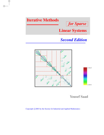
Iterative Methodsfor SparseLinear SystemsSecond Edition0.19E 070.10E-06Yousef SaadCopyright c 2003 by the Society for Industrial and Applied Mathematics
ContentsPrefacePreface to. second. . . . edition. . . . . . . . . . . . . . . . . . . . . . . . . . . . .Preface to. first. . edition. . . . . . . . . . . . . . . . . . . . . . . . . . . . . . .1 Background in Linear Algebra1.1Matrices . . . . . . . . . . . . . . . . . . . . . .1.2Square Matrices and Eigenvalues . . . . . . . . .1.3Types of Matrices . . . . . . . . . . . . . . . . .1.4Vector Inner Products and Norms . . . . . . . . .1.5Matrix Norms . . . . . . . . . . . . . . . . . . .1.6Subspaces, Range, and Kernel . . . . . . . . . . .1.7Orthogonal Vectors and Subspaces . . . . . . . .1.8Canonical Forms of Matrices . . . . . . . . . . .1.8.1Reduction to the Diagonal Form . . .1.8.2The Jordan Canonical Form . . . . .1.8.3The Schur Canonical Form . . . . .1.8.4Application to Powers of Matrices .1.9Normal and Hermitian Matrices . . . . . . . . . .1.9.1Normal Matrices . . . . . . . . . . .1.9.2Hermitian Matrices . . . . . . . . .1.10Nonnegative Matrices, M-Matrices . . . . . . . .1.11Positive-Definite Matrices . . . . . . . . . . . . .1.12Projection Operators . . . . . . . . . . . . . . . .1.12.1Range and Null Space of a Projector1.12.2Matrix Representations . . . . . . .1.12.3Orthogonal and Oblique Projectors .1.12.4Properties of Orthogonal Projectors .1.13Basic Concepts in Linear Systems . . . . . . . . .1.13.1Existence of a Solution . . . . . . .1.13.2Perturbation Analysis . . . . . . . 7383940412 Discretization of PDEs2.1Partial Differential Equations . . . . . . . . . . . . . . . . . .2.1.1Elliptic Operators . . . . . . . . . . . . . . . . .474747v.
CONTENTSvi2.22.32.42.52.1.2The Convection Diffusion Equation . . . . . . .Finite Difference Methods . . . . . . . . . . . . . . . . . . .2.2.1Basic Approximations . . . . . . . . . . . . . .2.2.2Difference Schemes for the Laplacean Operator2.2.3Finite Differences for 1-D Problems . . . . . . .2.2.4Upwind Schemes . . . . . . . . . . . . . . . .2.2.5Finite Differences for 2-D Problems . . . . . . .2.2.6Fast Poisson Solvers . . . . . . . . . . . . . . .The Finite Element Method . . . . . . . . . . . . . . . . . .Mesh Generation and Refinement . . . . . . . . . . . . . . .Finite Volume Method . . . . . . . . . . . . . . . . . . . . .3 Sparse Matrices3.1Introduction . . . . . . . . . . . . . . . . . . . .3.2Graph Representations . . . . . . . . . . . . . . .3.2.1Graphs and Adjacency Graphs . . . .3.2.2Graphs of PDE Matrices . . . . . . .3.3Permutations and Reorderings . . . . . . . . . . .3.3.1Basic Concepts . . . . . . . . . . . .3.3.2Relations with the Adjacency Graph3.3.3Common Reorderings . . . . . . . .3.3.4Irreducibility . . . . . . . . . . . . .3.4Storage Schemes . . . . . . . . . . . . . . . . . .3.5Basic Sparse Matrix Operations . . . . . . . . . .3.6Sparse Direct Solution Methods . . . . . . . . . .3.6.1Minimum degree ordering . . . . . .3.6.2Nested Dissection ordering . . . . .3.7Test Problems . . . . . . . . . . . . . . . . . . .4 Basic Iterative Methods4.1Jacobi, Gauss-Seidel, and SOR . . . . . . . . . . .4.1.1Block Relaxation Schemes . . . . . .4.1.2Iteration Matrices and Preconditioning4.2Convergence . . . . . . . . . . . . . . . . . . . . .4.2.1General Convergence Result . . . . . .4.2.2Regular Splittings . . . . . . . . . . .4.2.3Diagonally Dominant Matrices . . . .4.2.4Symmetric Positive Definite Matrices .4.2.5Property A and Consistent Orderings .4.3Alternating Direction Methods . . . . . . . . . . 979798.1051051081121141151181191221231275 Projection Methods1335.1Basic Definitions and Algorithms . . . . . . . . . . . . . . . . 1335.1.1General Projection Methods . . . . . . . . . . . . 134
CONTENTSvii.1351371371381401421421451471476 Krylov Subspace Methods Part I6.1Introduction . . . . . . . . . . . . . . . . . . . . . . . . .6.2Krylov Subspaces . . . . . . . . . . . . . . . . . . . . . .6.3Arnoldi’s Method . . . . . . . . . . . . . . . . . . . . . .6.3.1The Basic Algorithm . . . . . . . . . . . . . .6.3.2Practical Implementations . . . . . . . . . . .6.4Arnoldi’s Method for Linear Systems (FOM) . . . . . . . .6.4.1Variation 1: Restarted FOM . . . . . . . . . .6.4.2Variation 2: IOM and DIOM . . . . . . . . .6.5GMRES . . . . . . . . . . . . . . . . . . . . . . . . . . .6.5.1The Basic GMRES Algorithm . . . . . . . . .6.5.2The Householder Version . . . . . . . . . . .6.5.3Practical Implementation Issues . . . . . . . .6.5.4Breakdown of GMRES . . . . . . . . . . . .6.5.5Variation 1: Restarting . . . . . . . . . . . . .6.5.6Variation 2: Truncated GMRES Versions . . .6.5.7Relations between FOM and GMRES . . . . .6.5.8Residual smoothing . . . . . . . . . . . . . .6.5.9GMRES for complex systems . . . . . . . . .6.6The Symmetric Lanczos Algorithm . . . . . . . . . . . . .6.6.1The Algorithm . . . . . . . . . . . . . . . . .6.6.2Relation with Orthogonal Polynomials . . . .6.7The Conjugate Gradient Algorithm . . . . . . . . . . . . .6.7.1Derivation and Theory . . . . . . . . . . . . .6.7.2Alternative Formulations . . . . . . . . . . .6.7.3Eigenvalue Estimates from the CG Coefficients6.8The Conjugate Residual Method . . . . . . . . . . . . . .6.9GCR, ORTHOMIN, and ORTHODIR . . . . . . . . . . . .6.10The Faber-Manteuffel Theorem . . . . . . . . . . . . . . .6.11Convergence Analysis . . . . . . . . . . . . . . . . . . . .6.11.1Real Chebyshev Polynomials . . . . . . . . .6.11.2Complex Chebyshev Polynomials . . . . . . .6.11.3Convergence of the CG Algorithm . . . . . 5.25.35.45.1.2Matrix Representation . . . . . . . .General Theory . . . . . . . . . . . . . . . . . .5.2.1Two Optimality Results . . . . . . .5.2.2Interpretation in Terms of Projectors5.2.3General Error Bound . . . . . . . . .One-Dimensional Projection Processes . . . . . .5.3.1Steepest Descent . . . . . . . . . . .5.3.2Minimal Residual (MR) Iteration . .5.3.3Residual Norm Steepest Descent . .Additive and Multiplicative Processes . . . . . . .
CONTENTSviii6.126.11.4Convergence of GMRES . . . . . . . . . . . . . . 215Block Krylov Methods . . . . . . . . . . . . . . . . . . . . . 2187 Krylov Subspace Methods Part II7.1Lanczos Biorthogonalization . . . . . . . . . . .7.1.1The Algorithm . . . . . . . . . . . .7.1.2Practical Implementations . . . . . .7.2The Lanczos Algorithm for Linear Systems . . . .7.3The BCG and QMR Algorithms . . . . . . . . . .7.3.1The Biconjugate Gradient Algorithm7.3.2Quasi-Minimal Residual Algorithm .7.4Transpose-Free Variants . . . . . . . . . . . . . .7.4.1Conjugate Gradient Squared . . . . .7.4.2BICGSTAB . . . . . . . . . . . . .7.4.3Transpose-Free QMR (TFQMR) . .8 Methods Related to the Normal Equations8.1The Normal Equations . . . . . . . . . . . . . . . .8.2Row Projection Methods . . . . . . . . . . . . . .8.2.1Gauss-Seidel on the Normal Equations8.2.2Cimmino’s Method . . . . . . . . . .8.3Conjugate Gradient and Normal Equations . . . . .8.3.1CGNR . . . . . . . . . . . . . . . . .8.3.2CGNE . . . . . . . . . . . . . . . . .8.4Saddle-Point Problems . . . . . . . . . . . . . . . 2632662662672689 Preconditioned Iterations9.1Introduction . . . . . . . . . . . . . . . . . . . . . . . . .9.2Preconditioned Conjugate Gradient . . . . . . . . . . . . .9.2.1Preserving Symmetry . . . . . . . . . . . . .9.2.2Efficient Implementations . . . . . . . . . . .9.3Preconditioned GMRES . . . . . . . . . . . . . . . . . . .9.3.1Left-Preconditioned GMRES . . . . . . . . .9.3.2Right-Preconditioned GMRES . . . . . . . .9.3.3Split Preconditioning . . . . . . . . . . . . .9.3.4Comparison of Right and Left Preconditioning9.4Flexible Variants . . . . . . . . . . . . . . . . . . . . . . .9.4.1Flexible GMRES . . . . . . . . . . . . . . . .9.4.2DQGMRES . . . . . . . . . . . . . . . . . .9.5Preconditioned CG for the Normal Equations . . . . . . . .9.6The Concus, Golub, and Widlund Algorithm . . . . . . . .275275276276279282282284285285287287290291292.10 Preconditioning Techniques29710.1Introduction . . . . . . . . . . . . . . . . . . . . . . . . . . . 29710.2Jacobi, SOR, and SSOR Preconditioners . . . . . . . . . . . . 298
CONTENTS10.310.410.510.610.710.8ixILU Factorization Preconditioners . . . . . . . . . . . . .10.3.1Incomplete LU Factorizations . . . . . . . . .10.3.2Zero Fill-in ILU (ILU(0)) . . . . . . . . . . .10.3.3Level of Fill and ILU(p) . . . . . . . . . . . .10.3.4Matrices with Regular Structure . . . . . . . .10.3.5Modified ILU (MILU) . . . . . . . . . . . . .Threshold Strategies and ILUT . . . . . . . . . . . . . . .10.4.1The ILUT Approach . . . . . . . . . . . . . .10.4.2Analysis . . . . . . . . . . . . . . . . . . . .10.4.3Implementation Details . . . . . . . . . . . .10.4.4The ILUTP Approach . . . . . . . . . . . . .10.4.5The ILUS Approach . . . . . . . . . . . . . .10.4.6The Crout ILU Approach . . . . . . . . . . .Approximate Inverse Preconditioners . . . . . . . . . . . .10.5.1Approximating the Inverse of a Sparse Matrix10.5.2Global Iteration . . . . . . . . . . . . . . . .10.5.3Column-Oriented Algorithms . . . . . . . . .10.5.4Theoretical Considerations . . . . . . . . . .10.5.5Convergence of Self Preconditioned MR . . .10.5.6Approximate Inverses via bordering . . . . . .10.5.7Factored inverses via orthogonalization: AINV10.5.8Improving a Preconditioner . . . . . . . . . .Reordering for ILU . . . . . . . . . . . . . . . . . . . . .10.6.1Symmetric permutations . . . . . . . . . . . .10.6.2Nonsymmetric reorderings . . . . . . . . . . .Block Preconditioners . . . . . . . . . . . . . . . . . . . .10.7.1Block-Tridiagonal Matrices . . . . . . . . . .10.7.2General Matrices . . . . . . . . . . . . . . . .Preconditioners for the Normal Equations . . . . . . . . .10.8.1Jacobi, SOR, and Variants . . . . . . . . . . .10.8.2IC(0) for the Normal Equations . . . . . . . .10.8.3Incomplete Gram-Schmidt and ILQ . . . . . .11 Parallel Implementations11.1Introduction . . . . . . . . . . . . . . . . . . . . . . . .11.2Forms of Parallelism . . . . . . . . . . . . . . . . . . . .11.2.1Multiple Functional Units . . . . . . . . . .11.2.2Pipelining . . . . . . . . . . . . . . . . . .11.2.3Vector Processors . . . . . . . . . . . . . .11.2.4Multiprocessing and Distributed Computing11.3Types of Parallel Architectures . . . . . . . . . . . . . .11.3.1Shared Memory Computers . . . . . . . . .11.3.2Distributed Memory Architectures . . . . .11.4Types of Operations . . . . . . . . . . . . . . . . . . . 9369370370370371371371372374376
CONTENTSx11.511.6Matrix-by-Vector Products . . . . . . . . . . . . . . . . . .11.5.1The CSR and CSC Formats . . . . . . . . . . .11.5.2Matvecs in the Diagonal Format . . . . . . . . .11.5.3The Ellpack-Itpack Format . . . . . . . . . . .11.5.4The Jagged Diagonal Format . . . . . . . . . .11.5.5The Case of Distributed Sparse Matrices . . . .Standard Preconditioning Operations . . . . . . . . . . . . .11.6.1Parallelism in Forward Sweeps . . . . . . . . .11.6.2Level Scheduling: the Case of 5-Point Matrices11.6.3Level Scheduling for Irregular Graphs . . . . .12 Parallel Preconditioners12.1Introduction . . . . . . . . . . . . . . . . . . . . . . .12.2Block-Jacobi Preconditioners . . . . . . . . . . . . . .12.3Polynomial Preconditioners . . . . . . . . . . . . . . .12.3.1Neumann Polynomials . . . . . . . . . . .12.3.2Chebyshev Polynomials . . . . . . . . . .12.3.3Least-Squares Polynomials . . . . . . . .12.3.4The Nonsymmetric Case . . . . . . . . . .12.4Multicoloring . . . . . . . . . . . . . . . . . . . . . .12.4.1Red-Black Ordering . . . . . . . . . . . .12.4.2Solution of Red-Black Systems . . . . . .12.4.3Multicoloring for General Sparse Matrices12.5Multi-Elimination ILU . . . . . . . . . . . . . . . . . .12.5.1Multi-Elimination . . . . . . . . . . . . .12.5.2ILUM . . . . . . . . . . . . . . . . . . .12.6Distributed ILU and SSOR . . . . . . . . . . . . . . .12.7Other Techniques . . . . . . . . . . . . . . . . . . . .12.7.1Approximate Inverses . . . . . . . . . . .12.7.2Element-by-Element Techniques . . . . .12.7.3Parallel Row Projection Preconditioners .13 Multigrid Methods13.1Introduction . . . . . . . . . . . . . . . . .13.2Matrices and spectra of model problems . .13.2.1Richardson’s iteration . . . . .13.2.2Weighted Jacobi iteration . . .13.2.3Gauss-Seidel iteration . . . . .13.3Inter-grid operations . . . . . . . . . . . . .13.3.1Prolongation . . . . . . . . . .13.3.2Restriction . . . . . . . . . . .13.4Standard multigrid techniques . . . . . . . .13.4.1Coarse problems and smoothers13.4.2Two-grid cycles . . . . . . . 24428431432436436438439439441
13.513.613.713.4.3V-cycles and W-cycles . . . . .13.4.4Full Multigrid . . . . . . . . .Analysis for the two-grid cycle . . . . . . .13.5.1Two important subspaces . . .13.5.2Convergence analysis . . . . .Algebraic Multigrid . . . . . . . . . . . . .13.6.1Smoothness in AMG . . . . . .13.6.2Interpolation in AMG . . . . .13.6.3Defining coarse spaces in AMG13.6.4AMG via Multilevel ILU . . .Multigrid vs Krylov methods . . . . . . . .14 Domain Decomposition Methods14.1Introduction . . . . . . . . . . . . . . . . . . . . . . . . . . .14.1.1Notation . . . . . . . . . . . . . . . . . . . . . .14.1.2Types of Partitionings . . . . . . . . . . . . . . .14.1.3Types of Techniques . . . . . . . . . . . . . . . .14.2Direct Solution and the Schur Complement . . . . . . . . . . .14.2.1Block Gaussian Elimination . . . . . . . . . . . .14.2.2Properties of the Schur Complement . . . . . . .14.2.3Schur Complement for Vertex-Based Partitionings14.2.4Schur Complement for Finite-Element Partitionings14.2.5Schur Complement for the model problem . . . .14.3Schwarz Alternating Procedures . . . . . . . . . . . . . . . . .14.3.1Multiplicative Schwarz Procedure . . . . . . . . .14.3.2Multiplicative Schwarz Preconditioning . . . . . .14.3.3Additive Schwarz Procedure . . . . . . . . . . . .14.3.4Convergence . . . . . . . . . . . . . . . . . . . .14.4Schur Complement Approaches . . . . . . . . . . . . . . . . .14.4.1Induced Preconditioners . . . . . . . . . . . . . .14.4.2Probing . . . . . . . . . . . . . . . . . . . . . . .14.4.3Preconditioning Vertex-Based Schur Complements14.5Full Matrix Methods . . . . . . . . . . . . . . . . . . . . . . .14.6Graph Partitioning . . . . . . . . . . . . . . . . . . . . . . . .14.6.1Basic Definitions . . . . . . . . . . . . . . . . . .14.6.2Geometric Approach . . . . . . . . . . . . . . . .14.6.3Spectral Techniques . . . . . . . . . . . . . . . .14.6.4Graph Theory Techniques . . . . . . . . . . . . 504505506507References514Index535
xiiCONTENTS
Preface to the second editionIn the six years that passed since the publication of the first edition of this book,iterative methods for linear systems have made good progress in scientific and engineering disciplines. This is due in great part to the increased complexity and size ofthe new generation of linear and nonlinear systems which arise from typical applications. At the same time, parallel computing has penetrated the same applicationareas, as inexpensive computer power became broadly available and standard communication languages such as MPI gave a much needed standardization. This hascreated an incentive to utilize iterative rather than direct solvers because the problems solved are typically from 3-dimensional models for which direct solvers oftenbecome ineffective. Another incentive is that iterative methods are far easier to implement on parallel computers,Though iterative methods for linear systems have seen a significant maturation,there are still many open problems. In particular, it still cannot be stated that anarbitrary sparse linear system can be solved iteratively in an efficient way. If physicalinformation about the problem can be exploited, more effective and robust methodscan be tailored for the solutions. This strategy is exploited by multigrid methods. Inaddition, parallel computers necessitate different ways of approaching the problemand solution algorithms that are radically different from classical ones.Several new texts on the subject of this book have appeared since the first edition.Among these, are the books by Greenbaum [154], and Meurant [209]. The exhaustive5-volume treatise by G. W. Stewart [274] is likely to become the de-facto referencein numerical linear algebra in years to come. The related multigrid literature hasalso benefited from a few notable additions, including a new edition of the excellent“Multigrid tutorial” [65], and a new title by Trottenberg et al. [286].Most notable among the changes from the first edition, is the addition of a sorelyneeded chapter on Multigrid techniques. The chapters which have seen the biggestchanges are Chapter 3, 6, 10, and 12. In most cases, the modifications were made toupdate the material by adding topics that were developed recently or gained importance in the last few years. In some instances some of the older topics were removedor shortened. For example the discussion on parallel architecture has been shortened. In the mid-1990’s hypercubes and “fat-trees” were important topic to teach.This is no longer the case, since manufacturers have taken steps to hide the topologyfrom the user, in the sense that communication has become much less sensitive to thexiii
xivPREFACEunderlying architecture.The bibliography has been updated to include work that has appeared in the lastfew years, as well as to reflect change of emphasis when new topics have gainedimportance. Similarly, keeping in mind the educational side of this book, manynew exercises have been added. The first edition suffered many typographical errorswhich have been corrected. Many thanks to those readers who took the time to pointout errors.I would like to reiterate my thanks to all my colleagues who helped make thethe first edition a success (see the preface to the first edition). I received supportand encouragement from many students and colleagues to put together this revisedvolume. I also wish to thank those who proofread this book. I found that one ofthe best way to improve clarity is to solicit comments and questions from studentsin a course which teaches the material. Thanks to all students in Csci 8314 whohelped in this regard. Special thanks to Bernie Sheeham, who pointed out quite afew typographical errors and made numerous helpful suggestions.My sincere thanks to Michele Benzi, Howard Elman, and Steve Mc Cormickfor their reviews of this edition. Michele proof-read a few chapters thoroughly andcaught a few misstatements. Steve Mc Cormick’s review of Chapter 13 helped ensurethat my slight bias for Krylov methods (versus multigrid) was not too obvious. Hiscomments were at the origin of the addition of Section 13.7 (Multigrid vs Krylovmethods).I would also like to express my appreciation to the SIAM staff, especially LindaThiel and Sara Murphy.
PREFACExvSuggestions for teachingThis book can be used as a text to teach a graduate-level course on iterative methodsfor linear systems. Selecting topics to teach depends on whether the course is taughtin a mathematics department or a computer science (or engineering) department, andwhether the course is over a semester or a quarter. Here are a few comments on therelevance of the topics in each chapter.For a graduate course in a mathematics department, much of the material inChapter 1 should be known already. For non-mathematics majors most of the chapter must be covered or reviewed to acquire a good background for later chapters.The important topics for the rest of the book are in Sections: 1.8.1, 1.8.3, 1.8.4, 1.9,1.11. Section 1.12 is best treated at the beginning of Chapter 5. Chapter 2 is essentially independent from the rest and could be skipped altogether in a quarter session,unless multigrid methods are to be included in the course. One lecture on finite differences and the resulting matrices would be enough for a non-math course. Chapter3 aims at familiarizing the student with some implementation issues associated withiterative solution procedures for general sparse matrices. In a computer science orengineering department, this can be very relevant. For mathematicians, a mentionof the graph theory aspects of sparse matrices and a few storage schemes may besufficient. Most students at this level should be familiar with a few of the elementaryrelaxation techniques covered in Chapter 4. The convergence theory can be skippedfor non-math majors. These methods are now often used as preconditioners and thismay be the only motive for covering them.Chapter 5 introduces key concepts and presents projection techniques in general terms. Non-mathematicians may wish to skip Section 5.2.3. Otherwise, it isrecommended to start the theory section by going back to Section 1.12 on generaldefinitions on projectors. Chapters 6 and 7 represent the heart of the matter. It isrecommended to describe the first algorithms carefully and put emphasis on the factthat they generalize the one-dimensional methods covered in Chapter 5. It is alsoimportant to stress the optimality properties of those methods in Chapter 6 and thefact that these follow immediately from the properties of projectors seen in Section1.12. Chapter 6 is rather long and the instructor will need to select what to coveramong the non-essential topics as well as topics for reading.When covering the algorithms in Chapter 7, it is crucial to point out the maindifferences between them and those seen in Chapter 6. The variants such as CGS,BICGSTAB, and TFQMR can be covered in a short time, omitting details of thealgebraic derivations or covering only one of the three. The class of methods basedon the normal equation approach, i.e., Chapter 8, can be skipped in a math-orientedcourse, especially in the case of a quarter system. For a semester course, selectedtopics may be Sections 8.1, 8.2, and 8.4.Preconditioning is known to be the determining ingredient in the success of iterative methods in solving real-life problems. Therefore, at least some parts of Chapter9 and Chapter 10 should be covered. Section 9.2 and (very briefly) 9.3 are recommended. From Chapter 10, discuss the basic ideas in Sections 10.1 through 10.3.
PREFACExviThe rest could be skipped in a quarter course.Chapter 11 may be useful to present to computer science majors, but may beskimmed through or skipped in a mathematics or an engineering course. Parts ofChapter 12 could be taught primarily to make the students aware of the importanceof “alternative” preconditioners. Suggested selections are: 12.2, 12.4, and 12.7.2 (forengineers).Chapters 13 and 14 present important research areas and are primarily gearedto mathematics majors. Computer scientists or engineers may cover this material inless detail.To make these suggestions more specific, the following two tables are offeredas sample course outlines. Numbers refer to sections in the text. A semester courserepresents approximately 30 lectures of 75 minutes each whereas a quarter courseis approximately 20 lectures of 75 minutes each. Different topics are selected for amathematics course and a non-mathematics course.Semester courseWeeksMathematicsComputer Science / Eng.1–31.9 –1.132.1 – 2.53.1 – 3.31.1 – 1.6 (Read) ; 1.7; 1.9;1.11; 1.12; 2.1 – 2.23.1 – 3.64–64.1 – 4.25. 1 – 5.3; 6.1 – 6.46.5.1; 6.5.3 – 6.5.94.1 – 4.2.1; 4.2.35.1 – 5.2.1; 5.36.1 – 6.4; 6.5.1 – 6.5.57–96.6 – 6.86.9 – 6.11; 7.1 – 7.37.4.1; 7.4.2; 7.4.3 (Read)6.7.1 6.8–6.96.11.3; 7.1 – 7.37.4.1 – 7.4.2; 7.4.3 (Read)10 – 128.1; 8.2 ; 9.1 – 9.4;10.1 – 10.3; 10.4.1;10.5.1 – 10.5.78.1 – 8.3; 9.1 – 9.310.1 – 10.3 ; 10.4.1 – 10.4.3;10.5.1 – 10.5.4; 10.5.713 – 1512.2 – 12.413.1 – 13.514.1 – 14.611.1 – 11.4 (Read); 11.5 – 11.612.1 – 12.2 ; 12.4 – 12.714.1 – 14.3; 14.6
PREFACExviiQuarter courseWeeksMathematicsComputer Science / Eng.1–21.9 – 1.134.1 – 4.2; 5.1 – 5.41.1 – 1.6 (Read); 3.1 – 3.54.1; 1.12 (Read)3–46.1 – 6.46.5.1; 6.5.3 – 6.5.55.1 – 5.2.1; 5.36.1 – 6.35–66.7.1; 6.11.3; 7.1 – 7.37.4.1 – 7.4.2; 7.4.3 (Read)6.4; 6.5.1; 6.5.3 – 6.5.56.7.1; 6.11.3; 7.1 – 7.37–89.1 – 9.310.1 – 10.3; 10.5.1; 10.5.77.4.1 – 7.4.2 (Read); 9.1 – 9.310.1 – 10.3; 10.5.1; 10.5.79 – 1013.1 – 13.514.1 – 14.411.1 – 11.4 (Read); 11.5; 11.612.1 – 12.2; 12.4 – 12.7
xviiiPREFACE
Preface to the first editionIterative methods for solving general, large sparse linear systems have been gaining popularity in many areas of scientific computing. Until recently, direct solutionmethods were often preferred to iterative methods in real applications because oftheir robustness and predictable behavior. However, a number of efficient iterativesolvers were discovered and the increased need for solving very large linear systemstriggered a noticeable and rapid shift toward iterative techniques in many applications.This trend can be traced back to the 1960s and 1970s when two important developments revolutionized solution methods for large linear systems. First was therealization that one can take advantage of “sparsity” to design special direct methods that can be quite economical. Initiated by electrical engineers, these “directsparse solution methods” led to the development of reliable and efficient general-purpose direct solution software codes over the next three decades. Second wasthe emergence of preconditioned conjugate gradient-like methods for solving linearsystems. It was found that the combination of preconditioning and Krylov subspaceiterations could provide efficient and simple “general-purpose” procedures that couldcompete with direct solvers. Preconditioning involves exploiting ideas from sparsedirect solvers. Gradually, iterative methods started to approach the quality of direct solvers. In earlier times, iterative methods were often special-purpose in nature.They were developed with certain applications in mind, and their efficiency relied onmany problem-dependent parameters.Now, three-dimensional models are commonplace and iterative methods are almost mandatory. The memory and the computational requirements for solving threedimensional Partial Differential Equations, or two-dimensional ones involving manydegrees of freedom per point, may seriously challenge the most efficient direct solversavailable today. Also, iterative methods are gaining ground because they are easierto implement efficiently on high-performance computers than direct methods.My intention in writing this volume is to provide up-to-date coverage of iterative methods for solving large sparse linear systems. I focused the book on practicalmethods that work for general sparse matrices rather than for any specific class ofproblems. It is indeed becoming important to embrace applications not necessarily governed by Partial Differential Equations, as these applications are on the rise.xix
xxPREFACEApart from two recent volumes by Axelsson [14] and Hackbusch [163], few books oniterative methods have appeared since the excellent ones by Varga [293]. and laterYoung [322]. Since then, researchers and practitioners have achieved remarkableprogress in the development and use of effective iterative methods. Unfortunately,fewer elegant results have been discovered since the 1950s and 1960s. The field hasmoved in other directions. Methods have gained not only in efficiency but also inrobustness and in generality. The traditional techniques which required rather complicated procedures to determine optimal acceleration parameters have yielded to theparameter-free conjugate gradient class of methods.The primary aim of this book is to describe some of the best techniques availabletoday, from both preconditioners and accelerators. One of the aims of the book isto provide a good mix of theory and practice. It also addresses some of the currentresearch issues such as parallel implementations and robust preconditioners. Theemphasis is on Krylov subspace methods, currently the most practical and commongroup of techniques used in applications. Although there is a tutorial chapter thatcovers the discretization of Partial Differential Equations, the book is not biasedtoward any specific application area. Instead, the matrices are assumed to be generalsparse, possibly irregularly structured.The book has been structured in four distinct parts. The first part, Chapters 1 to 4,presents the basic tools. The second part, Chapters 5 to 8, presents projection methods and Krylov subspace techniques. The third part, Chapters 9 and 10, discussespreco
Contents Preface xiii Preface to second edition. . . . . . . . . . . . . . . . . . . . . . . . . . . . . . . . . . xiii Preface to first edition .
