WIXLIB

CONTENTS717 Linear Transformations17.1 Matrix Multiplication As A Linear Transformation . . . . .17.2 L (V, W ) As A Vector Space . . . . . . . . . . . . . . . . . .17.3 Eigenvalues And Eigenvectors Of Linear Transformations .17.4 Block Diagonal Matrices . . . . . . . . . . . . . . . . . . . .17.5 The Matrix Of A Linear Transformation . . . . . . . . . . .17.5.1 Some Geometrically Defined Linear Transformations17.5.2 Rotations About A Given Vector . . . . . . . . . . .17.6 Exercises . . . . . . . . . . . . . . . . . . . . . . . . . . . .369369369370375379386386388A The Jordan Canonical Form*391B The Fundamental Theorem Of Algebra399C Answers To Selected ExercisesC.1 Exercises 21 . . . . . . . . . .C.2 Exercises 36 . . . . . . . . . .C.3 Exercises 47 . . . . . . . . . .C.4 Exercises 56 . . . . . . . . . .C.5 Exercises 72 . . . . . . . . . .C.6 Exercises 92 . . . . . . . . . .C.7 Exercises 111 . . . . . . . . .C.8 Exercises 158 . . . . . . . . .C.9 Exercises 175 . . . . . . . . .C.10 Exercises 190 . . . . . . . . .C.11 Exercises 214 . . . . . . . . .C.12 Exercises 239 . . . . . . . . .C.13 Exercises 276 . . . . . . . . .C.14 Exercises 296 . . . . . . . . .C.15 Exercises 322 . . . . . . . . .C.16 Exercises 326 . . . . . . . . .C.17 Exercises 345 . . . . . . . . .C.18 Exercises 363 . . . . . . . . .C.19 Exercises 388 . . . . . . . . .c 2011,Copyright 19419420421426Download a free pdf of this book at: r-algebra or at http://www.saylor.org/courses/ma211/

8This page left blank intentionally.Download a free pdf of this book at: r-algebra or at http://www.saylor.org/courses/ma211/

PrefaceThis is an introduction to linear algebra. The main part of the book features row operations andeverything is done in terms of the row reduced echelon form and specific algorithms. At the end, themore abstract notions of vector spaces and linear transformations on vector spaces are presented.However, this is intended to be a first course in linear algebra for students who are sophomoresor juniors who have had a course in one variable calculus and a reasonable background in collegealgebra. I have given complete proofs of all the fundamental ideas, but some topics such as Markovmatrices are not complete in this book but receive a plausible introduction. The book contains acomplete treatment of determinants and a simple proof of the Cayley Hamilton theorem althoughthese are optional topics. The Jordan form is presented as an appendix. I see this theorem as thebeginning of more advanced topics in linear algebra and not really part of a beginning linear algebracourse. There are extensions of many of the topics of this book in my on line book [11]. I have alsonot emphasized that linear algebra can be carried out with any field although there is an optionalsection on this topic, most of the book being devoted to either the real numbers or the complexnumbers. It seems to me this is a reasonable specialization for a first course in linear algebra.Linear algebra is a wonderful interesting subject. It is a shame when it degenerates into nothingmore than a challenge to do the arithmetic correctly. It seems to me that the use of a computeralgebra system can be a great help in avoiding this sort of tedium. I don’t want to over emphasizethe use of technology, which is easy to do if you are not careful, but there are certain standardthings which are best done by the computer. Some of these include the row reduced echelon form,P LU factorization, and QR factorization. It is much more fun to let the machine do the tediouscalculations than to suffer with them yourself. However, it is not good when the use of the computeralgebra system degenerates into simply asking it for the answer without understanding what theoracular software is doing. With this in mind, there are a few interactive links which explain howto use a computer algebra system to accomplish some of these more tedious standard tasks. Theseare obtained by clicking on the symbol I. I have included how to do it using maple and scientificnotebook because these are the two systems I am familiar with and have on my computer. Othersystems could be featured as well. It is expected that people will use such computer algebra systemsto do the exercises in this book whenever it would be helpful to do so, rather than wasting hugeamounts of time doing computations by hand. However, this is not a book on numerical analysis sono effort is made to consider many important numerical analysis issues.9Download a free pdf of this book at: r-algebra or at http://www.saylor.org/courses/ma211/

10This page left blank intentionallyDownload a free pdf of this book at: r-algebra or at http://www.saylor.org/courses/ma211/

Some Prerequisite TopicsThe reader should be familiar with most of the topics in this chapter. However, it is often the casethat set notation is not familiar and so a short discussion of this is included first. Complex numbersare then considered in somewhat more detail. Many of the applications of linear algebra require theuse of complex numbers, so this is the reason for this introduction.1.1Sets And Set NotationA set is just a collection of things called elements. Often these are also referred to as points incalculus. For example {1, 2, 3, 8} would be a set consisting of the elements 1,2,3, and 8. To indicatethat 3 is an element of {1, 2, 3, 8} , it is customary to write 3 {1, 2, 3, 8} . 9 / {1, 2, 3, 8} means 9 isnot an element of {1, 2, 3, 8} . Sometimes a rule specifies a set. For example you could specify a setas all integers larger than 2. This would be written as S {x Z : x 2} . This notation says: theset of all integers, x, such that x 2.If A and B are sets with the property that every element of A is an element of B, then A is a subsetof B. For example, {1, 2, 3, 8} is a subset of {1, 2, 3, 4, 5, 8} , in symbols, {1, 2, 3, 8} {1, 2, 3, 4, 5, 8} .It is sometimes said that “A is contained in B” or even “B contains A”. The same statement aboutthe two sets may also be written as {1, 2, 3, 4, 5, 8} {1, 2, 3, 8}.The union of two sets is the set consisting of everything which is an element of at least one ofthe sets, A or B. As an example of the union of two sets {1, 2, 3, 8} {3, 4, 7, 8} {1, 2, 3, 4, 7, 8}because these numbers are those which are in at least one of the two sets. In generalA B {x : x A or x B} .Be sure you understand that something which is in both A and B is in the union. It is not anexclusive or.The intersection of two sets, A and B consists of everything which is in both of the sets. Thus{1, 2, 3, 8} {3, 4, 7, 8} {3, 8} because 3 and 8 are those elements the two sets have in common. Ingeneral,A B {x : x A and x B} .The symbol [a, b] where a and b are real numbers, denotes the set of real numbers x, such thata x b and [a, b) denotes the set of real numbers such that a x b. (a, b) consists of the set ofreal numbers x such that a x b and (a, b] indicates the set of numbers x such that a x b.[a, ) means the set of all numbers x such that x a and ( , a] means the set of all real numberswhich are less than or equal to a. These sorts of sets of real numbers are called intervals. The twopoints a and b are called endpoints of the interval. Other intervals such as ( , b) are defined byanalogy to what was just explained. In general, the curved parenthesis indicates the end point itsits next to is not included while the square parenthesis indicates this end point is included. Thereason that there will always be a curved parenthesis next to or is that these are not realnumbers. Therefore, they cannot be included in any set of real numbers.11Download a free pdf of this book at: r-algebra or at http://www.saylor.org/courses/ma211/

12SOME PREREQUISITE TOPICSA special set which needs to be given a name is the empty set also called the null set, denotedby . Thus is defined as the set which has no elements in it. Mathematicians like to say the emptyset is a subset of every set. The reason they say this is that if it were not so, there would have toexist a set A, such that has something in it which is not in A. However, has nothing in it and sothe least intellectual discomfort is achieved by saying A.If A and B are two sets, A \ B denotes the set of things which are in A but not in B. ThusA \ B {x A : x / B} .Set notation is used whenever convenient.To illustrate the use of this notation relative to intervals consider three examples of inequalities.Their solutions will be written in the notation just described.Example 1.1.1 Solve the inequality 2x 4 xx 812 is the answer. This is written in terms of an interval as ( , 12].Example 1.1.2 Solve the inequality (x 1) (2xThe solution is x 1 or x 3) 0.33. In terms of set notation this is denoted by ( , 1] [ , ).22Example 1.1.3 Solve the inequality x (x 2) 4.This is true for any value of x. It is written as R or ( , ) .1.2FunctionsThe concept of a function is that of something which gives a unique output for a given input.Definition 1.2.1 Consider two sets, D and R along with a rule which assigns a unique elementof R to every element of D. This rule is called a function and it is denoted by a letter such as f.Given x D, f (x) is the name of the thing in R which results from doing f to x. Then D is calledthe domain of f. In order to specify that D pertains to f , the notation D (f ) may be used. Theset R is sometimes called the range of f. These days it is referred to as the codomain. The set ofall elements of R which are of the form f (x) for some x D is therefore, a subset of R. This issometimes referred to as the image of f . When this set equals R, the function f is said to be onto,also surjective. If whenever x ̸ y it follows f (x) ̸ f (y), the function is called one to one., also injective It is common notation to write f : D R to denote the situation just describedin this definition where f is a function defined on a domain D which has values in a codomain R.fSometimes you may also see something like D R to denote the same thing.Example 1.2.2 Let D consist of the set of people who have lived on the earth except for Adam andfor d D, let f (d) the biological father of d. Then f is a function.This function is not the sort of thing studied in calculus but it is a function just the same.Example 1.2.3 Consider the list of numbers {1, 2, 3, 4, 5, 6, 7} D. Define a function which assignsan element of D to R {2, 3, 4, 5, 6, 7, 8} by f (x) x 1 for each x D.This function is onto because every element of R is the result of doing f to something in D. Thefunction is also one to one. This is because if x 1 y 1, then it follows x y. Thus differentelements of D must go to different elements of R.In this example there was a clearly defined procedure which determined the function. However,sometimes there is no discernible procedure which yields a particular function.Download a free pdf of this book at: r-algebra or at http://www.saylor.org/courses/ma211/

1.3. GRAPHS OF FUNCTIONS13Example 1.2.4 Consider the ordered pairs, (1, 2) , (2, 2) , (8, 3) , (7, 6) and letD {1, 2, 8, 7} ,the set of first entries in the given set of ordered pairs and letR {2, 2, 3, 6} ,the set of second entries, and let f (1) 2, f (2) 2, f (8) 3, and f (7) 6.This specifies a function even though it does not come from a convenient formula.1.3Graphs Of FunctionsRecall the notion of the Cartesian coordinate system you probably saw earlier. It involved an x axis,a y axis, two lines which intersect each other at right angles and one identifies a point by specifying apair of numbers. For example, the number (2, 3) involves going 2 units to the right on the x axis andthen 3 units directly up on a line perpendicular to the x axis. For example, consider the followingpicture.y6(2, 3)-xBecause of the simple correspondence between points in the plane and the coordinates of a pointin the plane, it is often the case that people are a little sloppy in referring to these things. Thus, itis common to see (x, y) referred to as a point in the plane. In terms of relations, if you graph thepoints as just described, you will have a way of visualizing the relation.The reader has likely encountered the notion of graphing relations of the form y 2x 3 ory x2 5. The meaning of such an expression in terms of defining a relation is as follows. Therelation determined by the equation y 2x 3 means the set of all ordered pairs (x, y) which arerelated by this formula. Thus the relation can be written as{(x, y) : y 2x 3} .2The relation determined by y x 5 is{}(x, y) : y x2 5 .Note that these relations are also functions. For the first, you could let f (x) 2x 3 and this wouldtell you a rule which tells what the function does to x. However, some relations are not functions.For example, you could consider x2 y 2 1. Written more formally, the relation it defines is{}(x, y) : x2 y 2 1Now if you give a value for x, there might be two values for y which are associated with the givenvalue for x. In fact y 1 x2Thus this relation would not be a function.Download a free pdf of this book at: r-algebra or at http://www.saylor.org/courses/ma211/

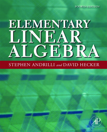
14SOME PREREQUISITE TOPICSRecall how to graph a relation. You first found lots of ordered pairs which satisfied the relation.For example (0, 3),(1, 5), and ( 1, 1) all satisfy y 2x 3 which describes a straight line. Thenyou connected them with a curve. Here are some simple examples which you should see that youunderstand. First here is the graph of y x2 1.54321–20–112–1Now here is the graph of the relation y 2x 1 which is a straight line.54321–20–112–1Sometimes a relation is defined using different formulas depending on the location of one of thevariables. For example, consider x

Elementary Linear Algebra was written by Dr. Kenneth Kuttler of Brigham Young University for teaching Linear Algebra I. After The Saylor Foundation accepted his submission to Wave I of the Open Textbook Challenge, this textbook was relicensed as CC-BY 3.0