Transcription
Honor’s Thesis:Portfolio Construction &Modern Portfolio TheoryMarinella PiñateB.S. in Industrial and Systems EngineeringGraduation Term: Fall 2013Honor’s Status: Magna Cum Laude&Oscar OropezaB.S. in Industrial and Systems EngineeringGraduation Term: Fall 2013Honor’s Status: Magna Cum Laude
Table of ContentsAbstract . 2Introduction . 2Investment Management . 3Portfolio Selection and the Markowitz Model . 4Model Inputs . 7Model Limitations. 7Alternatives to the Markowitz Model . 8Asset Allocation vs. Equity Portfolio Optimization . 9Methodology . 9Example Program. 12Limitations of Program . 18Conclusion . 19References . 20Page 1 of 20
AbstractThe purpose of this project is to explain the Modern Portfolio Theory, how it can be used, andillustrate an example by analyzing a hypothetical portfolio using Microsoft Excel with macros.To do this, it is important to understand the characteristics of the Markowitz model and howquadratic programming can be used to optimize this model. It is our goal that with this thesis, thebasic knowledge of investment can be expanded, as well as to outline the fact that manymathematical models used in operations research and other engineering fields can be usedextensively in other fields such as finance.IntroductionThe mean-variance portfolio selection is one of the cornerstones of modern portfolio theory. Thistheory attempts to maximize the expected return of a portfolio given a certain level of portfoliorisk, or equivalently attempts to minimize the portfolio’s risk given a certain level of expectedreturn. Its goal is to lower the risk by diversifying a portfolio of assets rather than investing inany individual asset. Harry Markowitz, a University of Chicago graduate student introduced thistheory in an 1952 article and in a 1958 book, after a stockbroker suggested him to study the stockmarket. He later received a share of the 1990 Nobel Prize in Economics for the introduction ofthis theory. Today, this theory is widely used in the fields of finance, investment, and operationsresearch.The goal of this paper is to explicitly explain the mean-variance model of the modern portfoliotheory along with the concept of quadratic programming and how they are used together tooptimize the selection of investment portfolios. It is worth noting that even though this theory,just as any other theory, has its own limitations; it is still considered to be the best way ofconstructing the most efficient investment portfolio that allows for the maximization of expectedreturn and minimization of risk.Page 2 of 20
Investment ManagementTo understand the concept of modern portfolio theory and portfolio analysis, it is important tounderstand the concept of Investment Management. This concept involves five steps. These are:1. Setting investment objectivesThis includes an analysis of the investment objectives of the investor whose funds are beingmanaged. This involves institutional investors (pension funds, insurance companies, mutualfunds, government agencies), and/or individual investors.2. Establishing an investment policy to satisfy investment objectivesThis step begins with asset allocation decisions, which means that a decision must be madeas to how the funds will be allocated among different classes of assets. Asset classes includea variety of investment products, such as:i.Equities or common stocks – These include large, medium, and small capitalizationstocks, and growth, value, domestic, foreign and emerging markets stocks.ii.Fixed income securities or bonds – These include treasury, municipal, corporate, highyield, mortgage backed securities, asset backed securities, and domestic, foreign, andemerging market bonds.iii.Cash – Includes T-Bills, money market, savingsiv.Alternatives – These alternative investments include commodities, real state,currencies, private equity, and hedge funds.In the development of an investment policy it is important to consider client, and regulatoryconstraints, as well as tax and accounting issues.3. Selecting an investment strategyPortfolio strategy can be classified as active or passive. Active portfolio strategy usesavailable information and forecasting techniques to seek a better performance than a portfoliothat is simply diversified broadly. In contrast, passive portfolio strategy involves minimalinputs; instead it relies on diversification to match the performance of some market index. Itassumes that the marketplace will reflect all available information in the price paid forsecurities. In the bond space, a structured portfolio strategy has also been used, in which aportfolio is designed to achieve the performance of some predetermined liabilities that mustbe paid out. The question now becomes, which investment strategy must be selected? AndPage 3 of 20
the answer depends on the client’s view of how price efficient the market is, the client’stolerance to risk, and the nature of the client’s liabilities.4. Selecting the specific assetsThis step attempts to construct an efficient portfolio, which is described as a portfolio thatprovides the greatest expected return for a given level of risk, or the lowest risk for a givenexpected return. For this step, three key inputs are required, these are: future expected return,variance of asset returns, and correlation of asset returns.5. Measuring and evaluating investment performanceThis involves measuring the performance of the portfolio and evaluating that performancerelative to some benchmark.Portfolio Selection and the Markowitz ModelThe goal of the portfolio selection is the construction of portfolios that maximize expectedreturns given a certain level of risk. Professor Harry Markowitz came up with a model thatattempts to do this by diversifying the portfolio. This model is called the Markowitz model or themean-variance model, because it attempts to maximize the mean (or expected return) of theentire portfolio, while reducing the variance as a measure of risk. This model shows that assetsshould not be selected individually, but rather as a portfolio, in order to reduce risk andmaximize expected return. For this, it is necessary to consider how each asset’s price changerelatively with the other assets in the portfolio. Portfolios that have the highest level of expectedreturn given a certain level of risk are called efficient portfolios. In order to construct theseportfolios, the Markowitz model makes five key assumptions. These are: Assumption 1: The expected return and the variance are the only parameters that affect aninvestor’s decision. Assumption 2: Investors are risk averse, meaning investors prefer investments with lowerrisks, given a certain level of expected return. Assumption 3: All investors’ goal is to achieve the highest level of expected return given acertain level of risk.Page 4 of 20
Assumption 4: All investors have the same expectations concerning expected return,variance, and covariance. Assumption 5: All investors have a one period investment horizon.After these assumptions are clear, portfolios can be constructed in a two-stage process: First, theinvestor needs to evaluate the available securities on the basis of their future perspectives toselect the best securities. Then, the investor needs to decide the allocation of current capital tothe chosen securities in order to meet investor’s policy, goals, and objectives.In order to calculate the actual return on a portfolio of assets over some period of time, thefollowing formula is used:Where, Rate of return of the portfolio Rate of return on asset g over the period weight of asset g in the portfolioG number of assets in the portfolioThus, the expected return from a portfolio of risky assets is calculated by:Where, the expected return of asset GTo quantify the concept of risk, Markowitz used the statistical measures of variance andcovariance. In order to measure the risk of a portfolio comprised of more than two assets, thefollowing formula is used:()()Page 5 of 20)
The variance of a portfolio not only depends on the variance of the assets but also upon thecovariance of any two assets, this is how closely the returns on every two assets in the portfoliomove with respect to each other, this is mainly due to the fact that financial markets interact,meaning that the investments do not vary independently. The covariance on any two assets canbe calculated as:()[][ [( )][][][( )] .( )]Where, the nth possible rate of return for asset i The nth possible rate of return for asset jp The probability of attaining the rate of return n for assets i andN the number of possible outcomes for the rate of returnA positive covariance means that the return on two assets move in the same direction, while anegative covariance means the returns tend to move in opposite directions. In order to have adiversified portfolio, a negative covariance is desired. This will allow investors to reduce theirexposure to individual asset risk, while allowing a desired expected return.In the same way, the correlation of two assets can be calculated in order to see the degree towhich two assets move together. Correlations show an easier way to evaluate behaviors.Correlations range from 1.0 to -1.0. A correlation of 1.0 means that there is perfect movementof the return of two assets in the same direction, while a correlation of -1.0 denotes a perfectmovement in opposite directions. In the other hand, a correlation of zero implies that the returnsare uncorrelated. Correlation can be defined as:(()Where,SD( Var(denotes standard deviation or.Page 6 of 20)
Model InputsIn order to use the mean-variance model for portfolio construction, one must obtain estimates ofthe return, variance and covariance for each investment of interest. When N stocks are evaluated,there will be N return and variance estimates, and [N(N-1)]/2 covariance estimates, making atotal of {2N [N(N-1)]/2} estimates. This tells us that even though this model is the mostcomprehensive and practical to use, it is of little use when solving problems with large numberof securities, because of the overwhelming amount of input estimates needed.Model LimitationsEven though the mean-variance theory is stable and has enhanced the portfolio managementprocess, it has some limitations to it. The disadvantages of the Markowitz model include: The effects of estimation error – Since the inputs of the model are created by analyzinghistorical data, they are considered estimates (expected returns, expected standarddeviations, and expected correlations), and thus contain some sort of error. This can causeover and under investment in certain assets, and make an efficient portfolio lookinefficient and an inefficient portfolio look efficient. To limit this error, constrainedoptimization can be used to set the maximum or minimum allocation of assets, andprevent assets with favorable inputs from dominating a portfolio. Unstable solutions – Small changes in inputs can lead to bigger changes in portfoliooutputs, thus making the result of this model unstable. Because of instability, an update toa small change in the expected return or standard deviation can lead to a differentportfolio allocation. To minimize these changes, a sensitivity analysis can be used; withthis analysis one can select an efficient portfolio and alter the inputs to see how close toefficient the portfolio is. The goal here is to identify a set of asset class weight that willbe close to efficient under different set of inputs. Reallocation costs – If there are two portfolios one with higher expected return than theother with the same risk level, one cannot simply alter one of the portfolio’s allocation tomatch the other, because depending on the asset classes within the portfolios and thePage 7 of 20
magnitude of the quantities involved, it might be costly to reallocate one portfolio tomatch the other’s expected return. It might be better to retain the current portfolioallocation despite its lack of efficiency.Alternatives to the Markowitz ModelDue to the Markowitz mean-variance model limitations, many authors have looked atalternatives for this model. However, other alternatives also have serious limitations of theirown. Other alternatives to the mean-variance model include: Non-variance risk measures –The semi-variance or semi-standard deviation of returnmeasures only returns below the mean because the variance of returns above it is notconsidered risk by investors. Utility function optimization – Maximizing expected utility of wealth is the basis ofrational decision making under uncertainty for many financial economists. The meanvariance theory is consistent with this only if any of the following two conditions holdtrue. 1) Asset returns are normally distributed, or 2) utility function is quadratic. Multi-period objectives – The mean-variance model is a single-period model forinvestment behavior. However, many investors have long-term horizons. To addressthese objectives, the mean-variance model can be based on long term units of time orconsider the multi-period distribution of the geometric mean of return. Monte Carlo financial planning – In this model, a computer model simulates the randomfunctioning of an investment and changes its liabilities over time. Linear programming optimizations – This is a special case of quadratic programming.The main difference is that linear programming excludes portfolio variance. To excludethe variance from the model, there are two things that can be done: 1) Set the objective tomaximize expected portfolio return subject to a variety of linear equality and inequalityconstraints on the structure of the portfolio, or 2) assume that the risk function is given bythe absolute deviation of the rate of return, and not the standard deviation as illustrated inthe Markowitz model.Page 8 of 20
Asset Allocation vs. Equity Portfolio OptimizationThe two most common uses of the mean-variance optimization theory involve asset allocationand equity portfolio optimization. In both cases, the objective is to find efficient allocations ofcapital to maximize expected return and minimize risk, subject to certain constraints. In assetallocation, there is a limited amount of risky assets usually less than 50 with a small number ofconstraints. The starting points for input estimates include sample means, variances, andcorrelations based on historic data.On the other hand, an equity portfolio optimization usually includes many securities. Domesticequity optimizations usually include 100-500 stocks, while international equity optimizationstypically include 4,000-5,000 stocks. These optimizations also include many constraints onportfolio characteristics, trading cost restrictions, and industry or sector membership. For thepurpose of this thesis, an asset allocation example has been made, and will be fully explained inthe following pages.MethodologyThe basis of the Markowitz model can be formulated by minimizing risk subject to a set ofconstraints, as noted below: Subject to: ̅ Page 9 of 20
In this case,represents the expected rate of return of asset i, ̅ is the minimum level of returnfor the portfolio chosen by the investor,is the covariance between assets i and j, andis thefraction (weight) of the portfolio invested in asset i.The first constraint specifies the minimum level of return the investor expects from the portfolio.The next constraint indicates that the sum of the weights of all assets invested must be equal tothe investment in the portfolio. The final constraint, the nonnegativity constraint, represents thatno short sales are allowed in the portfolio. To calculate this model and obtain the efficientfrontier, an understanding of quadratic programming is required.The objective of a quadratic program is a quadratic function of decision variables, and itsconstraints constitute linear functions of variables. In a Markowitz mean-variance portfoliooptimization problem the objective is the portfolio’s variance with linear constraints specifying alower bound for the portfolio’s return, as shown in the quadratic formulation above. Because oflinear constraints, quadratic programs have only one feasible region with an optimal solutionlying anywhere within the region. Quadratic programs can be either easy or extremely hard tosolve. The way of knowing this, is by seeing if the quadratic objective function and constraintsare convex or non-convex. If the objective is convex with a convex feasible region, then therewill be only one optimal solution, a globally optimal solution. However, if the objective functionand feasible region are non-convex, then it might have many locally optimal points, meaningthere are many more iterations to find a globally optimal solution, making the quadratic programdifficult to solve.The process knowing whether a quadratic program is convex or non-convex is beyond the scopeof this paper. For the purpose of this thesis, it is important to know that portfolio optimizationproblems are of quadratic objective functions that are convex, and this is why they are quadraticprograms that are easier to solve.With Markowitz’ optimization model and the ability to solve it using quadratic programming,one can construct an efficient frontier. This frontier is a set of efficient portfolios with the highestlevel of return for any given level of risk. It is an essential tool to see if the selected portfolio isPage 10 of 20
performing well, given a certain amount of risk. Portfolios that lie below the efficient frontier arenot efficient, because they do not provide enough return for the level of risk, while portfolios thatlie to the right are also inefficient, because they have a higher level of risk for the given rate ofreturn. The figure below depicts an example of an efficient frontier. The construction of anefficient frontier will be explained under the example program section.Figure 1: Efficient Frontier exampleThe red point in the above graph is called the global minimum variance (GMV) portfolio, whichis the portfolio with the highest expected return and the lowest risk. The green line in the abovegraph constitutes the capital allocation line (CAL). This line is an extension of the efficientfrontier that takes into account a risk-free asset. An example of a risk-free asset is a three-monthT-bill rate from the United States Treasury; this is because it is very unlikely that the USTreasury will default within the next three months.The tangency portfolio, where the CAL and efficient frontier cross, is considered to be the mostefficient portfolio out of all possible portfolios (assuming the same time horizon, risk, and returnlevels), since this portfolio maximizes the Sharpe ratio. The Sharpe ratio is a formula that tracksthe performance of a portfolio, taking into account the return of the portfolio, the return of therisk free asset, and the standard deviation (risk) of the portfolio. It tells the extra portfolio return,given a level of risk. The greater a portfolio’s Sharpe ratio, the better its performance. There isonly one most efficient portfolio (the tangency portfolio) where the Sharpe ratio is maximized,portfolios below or above the tangency portfolio decrease the Sharpe ratio. A negative SharpePage 11 of 20
ratio indicates that a risk-free asset would have better performance than the portfolio beinganalyzed. To calculate Sharpe ratio, the following formula is used:SR (̅̅̅)Where,̅ Expected portfolio return Risk free rate Portfolio Standard deviationThe rest of this paper will use the theory already explained to construct a portfolio usingMicrosoft Excel.Example ProgramTo show the capabilities of the Markowitz portfolio optimization model, an example portfoliowas created using Microsoft Excel. The purpose of this portfolio is to show an application of theMarkowitz theory. In addition, the following steps have been automated using macros to makethe program more user friendly. The only required inputs from the user are the historic monthlydata of the 15 stocks and the current 3-month Treasury bill monthly rate.The first step on the construction of the portfolio is to select 15 US stocks that represent differentsectors of the market. The companies that make up the list of chosen stocks for the purpose ofthis project are: AT&T, Ford Motor Co., Mondelez International, Inc., Interpublic Group of Cos.,Inc., Apple, Exxon Mobil, American Eagle Energy Corp., JP Morgan Chase & Co., TheGoldman Sachs Group, Laboratory Corp. of America Holdings, Wal-Mart Stores, Google,Southwest Airlines, and Atmos Energy Corp. The second step is to record the stock price permonth of each of these companies for a period of three years, from December 2009 to November2013. This data can be acquired from Yahoo Finance or any other finance website. The stockprice for each of the companies that make up the chosen portfolio are shown in the figure below.Page 12 of 20
Figure 2: Stock prices per month per companyIn the “Return %” tab of the Excel program, the percentage of expected return is calculated perstock per month using the natural logarithm function in excel. These expected returns along withtheir corresponding standard deviations, form the basis of the portfolio construction model. Thefigure below depicts the Return % tab.Figure 3: Percentage Expected Return per stockPage 13 of 20
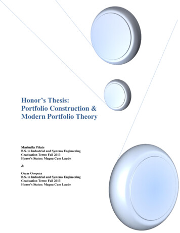
Next, the correlation and covariance matrices are calculated. These tables are constructed usingtheir corresponding functions in the “Matrices” tab and copied to the “Solver” tab. Thecovariance matrix shows the movement of stocks relative to each other to use in the analysis,while the correlation matrix shows an easier scale to visualize. The figure below shows thesolver tab with covariance and correlation matrices.Figure 4: Correlation and Covariance matricesFigure 4 also depicts two tables showing portfolio weights, these weights which have to sum to 1depict the percentage of assets that need to be invested in every stock of the portfolio to obtain anefficient portfolio. These cells are used in the solver part of the calculation.To find an efficient portfolio with quadratic objective function and linear constraints, the solveroption in excel had to be used. First the global minimum risk that returns the largest returnneeded to be defined. This is accomplished by relaxing the constraint for expected returns andadding the following data in the solver. Set Target Cell: Q 49 (This is the portfolio’s variance of return) Equal to: Min By Changing Cells: A 45: O 45 (These are the portfolio weights) Subject to the Constraints:o A 45: O 45 1Page 14 of 20
o A 45: O 45 0 (This is for no short selling.)o Q 45 1 (This makes sure our portfolio weight is always 100%, or notborrowing.)This returns the global minimum risk. Next, it is required to find the maximum return ignoringthe risk by entering the following data on the solver. Set Target Cell: Q 65(Portfolio’s expected return, ignoring variance) Equal to: Max By Changing Cells: A 45: O 45 (These are the portfolio weights.) Subject to the Constraints:o A 45: O 45 1o A 45: O 45 0 (This is for no short selling.)o Q 45 1 (This makes sure our portfolio weight is always 100%, or notborrowing.)This returns the best allocation of stocks to have the maximum return. It is important to note thatthe solver will allocate 100% of the funds to one stock (considered to be the one with higherexpected return) in general. This is a good way to quickly validate the work.In order to create an efficient frontier, we need the extreme points of the curve (the minimumrisk with the highest return and the highest return ignoring risk). Now add points in between byusing predetermined expected returns based of these extremes. In this example, predeterminedsteps were used to select risks. The following data was used to find one expected return to plotthe efficient frontier. Set Target Cell: Q 49 (This is the portfolio’s variance of return) Equal to: Min By Changing Cells: A 45: O 45 (These are the portfolio weights.) Subject to the Constraints:o A 45: O 45 1o A 45: O 45 0 (This is for no short selling.)Page 15 of 20
o Q 45 1 (This makes sure our portfolio weight is always 100 %.)o Q 65 B 79 (This sets a boundary on the expected return.)Finally, it is necessary to find the best Sharpe ratio for this portfolio to help create a CapitalAllocation Line. This can be done by entering the following information in the solver. Set Target Cell: D 68 [this is the Sharpe ratio: (Portfolio expected return - risk freeasset return)/Portfolio standard deviation of returns)] Equal to: Max By Changing Cells: A 45: O 45 (These are the portfolio weights.) Subject to the Constraints:o A 45: O 45 1o A 45: O 45 0 (This is for no short selling.)o Q 45 1 (This makes sure our portfolio weight is always 100 %.)Once all of these points are calculated, the table should look as the one below. Every result fromthe solver is showed with their respective weights (% holding) and each individual return perstock. These points are used to plot the efficient frontier as seen on Figure 1.Page 16 of 20
Figure 5 - Complete Data TableAll this information is summarized on the “Portfolio” tab with the name of the 15 companies,their industries, ticker symbol, calculated expected return, risk, % holding per stock and aweighted stock return. Additionally, there are three graphs to visualize the data. The first one isthe “Efficient Frontier” line graph of the given stocks. ext is the “Stock Return” bar graph thatdisplays the individual weighted return of a selected portfolio. Finally, the “% Holding” pie chartshow how your funds are allocated per company. On this tab, the user is able to choose a desiredportfolio return based on his or her risk tolerance. The data will dynamically adjust to the user’schoice.Page 17 of 20
Figure 6: Portfolio tabLimitations of ProgramEven though the example program is meant to be user friendly, there are still some limitations tothis program. The first limitation is the fact that the user can only input 15 stocks in the desiredportfolio and there must be 48 monthly data entries. The second limitation is that the “Solver”tab cannot be modified by the user because it will crash the program.Additionally, in order for the program to work, Microsoft Excel 2010 or a newer version may berequired. Another possible error may occur if the user does not have Excel solver installed on theExcel worksheet and enabled on the VB Developer console.To install the “Solver” functionality in Excel, select the Add-Ins option on the Excel's toolsmenu. If the solver option is shown on the list, check the box in front of its name. If the solveroption is not found, click Browse and navigate to the add-in file. After it appears on the add-inlist, select its checkbox. To set a reference to an add-in, the Solver must first be installed onPage 18 of 20
Excel. Next, on the VB Editor's Tools menu, select References. This lists all open workbooksand installed add-ins, as well as a list of resources installed on the host computer. Find “Solver”in the list, and check the box in front of its name.ConclusionTo conclude, this thesis has been focused on the Modern Portfolio theory and its cornerstones,the mean-variance model and the efficient frontier. The purpose is to explain the logic behindconstructing an efficient portfolio and how this model is facilitated by quadratic programming tofind the most efficient portfolio that minimizes the variance (risk) of the portfolio given a set oflinear constraints that specify a lower bound for portfolio return. We hope to use the acquiredknowledge on the creation of this thesis and Excel program as a foundation to expand onMarkowitz work in the near future, and become more knowledgeable investors. The mainlearning point of this thesis is that mathematical models and engineering can be used to modeland solve problems in any field with the right assumptions.Page 19 of 20
ReferencesPardalos, P. M., Athanasios Migdalas, and George Baourakis. Supply Chain and Finance.River Edge, NJ: World Scientific, 2004. Print.Fabozzi, Frank J., and H. Markowitz. The Theory and Practice of Investment Management.Hoboken, NJ: Wiley, 2002. Print.Benninga, Simon, and
Page 5 of 20 Assumption 4: All investors have the same expectations concerning expected return, variance, and covariance. Assumption 5: All investors have a one period investment horizon. After these assumptions are clear, portfolios can be constructed in a two-stage process: First, the investor needs to evaluate the available securities on the basis of their future perspectives to