Transcription
Unified Surface Analysis ManualWeather Prediction CenterOcean Prediction CenterNational Hurricane CenterHonolulu Forecast OfficeNovember 21, 2013
Table of ContentsChapter 1: Surface Analysis – Its History at the Analysis Centers .3Chapter 2: Datasets available for creation of the Unified Analysis . .5Chapter 3: The Unified Surface Analysis and related features. . .19Chapter 4: Creation/Merging of the Unified Surface Analysis . .24Chapter 5: Bibliography . .30Appendix A: Unified Graphics Legend showing Ocean Center symbols. . 332
Chapter 1:Surface Analysis – Its History at the Analysis Centers1. INTRODUCTIONSince 1942, surface analyses produced by several different offices within the U.S.Weather Bureau (USWB) and the National Oceanic and Atmospheric Administration’s(NOAA’s) National Weather Service (NWS) were generally based on the Norwegian CycloneModel (Bjerknes 1919) over land, and in recent decades, the Shapiro-Keyser Model over themid-latitudes of the ocean. The graphic below shows a typical evolution according to bothmodels of cyclone development.Conceptual models of cyclone evolution showing lower-tropospheric (e.g., 850-hPa) geopotential height andfronts (top), and lower-tropospheric potential temperature (bottom). (a) Norwegian cyclone model: (I)incipient frontal cyclone, (II) and (III) narrowing warm sector, (IV) occlusion; (b) Shapiro–Keyser cyclonemodel: (I) incipient frontal cyclone, (II) frontal fracture, (III) frontal T-bone and bent-back front, (IV)frontal T-bone and warm seclusion. Panel (b) is adapted from Shapiro and Keyser (1990) , their FIG. 10.27) to enhance the zonal elongation of the cyclone and fronts and to reflect the continued existence of thefrontal T-bone in stage IV. The stages in the respective cyclone evolutions are separated by approximately 6–24 h and the frontal symbols are conventional. The characteristic scale of the cyclones based on the distancefrom the geopotential height minimum, denoted by L, to the outermost geopotential height contour in stageIV is 1000 km.The National Meteorological Center (NMC) created Northern Hemisphere Surface Analysesfrom 1954 to 1996 from the equator to the North Pole, including adjacent ocean areas. TheWeather Prediction Center (WPC) and its predecessors have created North American SurfaceAnalyses since 1942. The Ocean Prediction Center (OPC) and its predecessors have created3
surface analyses since the 1970s for the open waters of the Atlantic and Pacific Oceans, north of18 degrees north. The Miami Weather Forecast Office and National Hurricane Center (NHC)composed surface analyses starting in 1942 for the waters of the Atlantic and much of the Pacificeast of Hawaii between the equator and the latitude of 500 N. The Weather Forecast OfficeHonolulu (HFO) performed surface analyses for the waters of the Pacific Ocean across thetropical, subtropical, and mid-latitudes sections of the northern Pacific south of 500 N and thetropical and subtropical sections of the southern Pacific north of 300 S. The Anchorage ForecastOffice (ANC) drew surface analyses for the northeast Pacific, eastern Asia, and the state ofAlaska for many years. This led to a significant duplication of effort over portions of theNorthern Hemisphere. Due to this redundancy, it was decided in 2001 that the various analysiscenters would limit their analyses to their areas of responsibilities (AOR) and would combine theanalyses from the other centers to create one seamless surface map for much of the NorthernHemisphere. This collaboration was intended to save each center time and concentrate morefully on their regions of expertise. By 2002, this plan went into place between NHC, OPC, andWPC, with HFO joining the collaboration effort in 2003.The WPC contributes a surface analysis covering the area from roughly 30 N to 85 Nlatitude, including much of mainland North America, the Canadian Archipelago, and the ArcticOcean. The Tropical Analysis and Forecast Branch (TAFB), part of the NHC, produces thesurface analysis portion covering the tropical and subtropical regions from the equator northwardto 31 N (except 30 N in the Pacific Ocean) from 20 E westward to 140 W, including overlandareas of Florida, Mexico, South America, Central America, Africa, and the Caribbean. The HFOgenerates analyses between 140 W westward to 130 E in the northern Pacific south of 30 N.OPC produces a pair of analyses for the Atlantic and Pacific oceans that span from NHC’s andHFO’s boundaries northward to Eastern Asia, the Aleutians, Greenland, Western Europe, and theMediterranean Sea. The two OPC analyses are split at the 1050W longitude between theirAtlantic and Pacific portions. All surface analyses are produced using the nAWIPS/Nmap2system. The analyses include all synoptic-scale systems and isobars every 4 millibars(mb)/hectopascals (hPa), while mesoscale features are depicted in the data-rich contiguousUnited States (CONUS) and in other locations where data permits. Intermediate isobars (every1-2 millibars/hectopascals) may be included in areas of weak pressure gradient in WPC, HFO,and NHC analyses. The usage of intermediate isobars is left to the analyst’s discretion based onthe pattern and value added to the analysis; aesthetics also may play a role. All surface analysesare saved, exchanged, and disseminated using a vector graphic format (VGF). The NWS unifiedsurface analysis involves extensive collaboration between OPC, NHC, WPC, and HFO(collectively referred to as the analysis centers.)A good surface analysis incorporates a variety of data sources to accurately depict thephysical processes occurring in the atmosphere at analysis time. Examples of the data sourcesinclude surface observations (including ship, fixed buoy and C-MAN, as well as those overland), satellite data, ocean surface winds as measured by scatterometer (ASCAT/OSCAT), andmodel analysis fields. Surface analyses are subjective in nature, and even skilled analysts canshow marked differences in their analyses (Uccellini et. al 1992). Through collaborationamongst the analysis centers, consistency with past analyses; and a review of the atmospheric4
models initializations, the Unified surface analyses provide NOAA’s National Weather Service(NWS) customers and users with the best consensus and consistent “one NWS” surface analyses.Chapter 2:Datasets available for creation of the Unified Analysis1. COMMON DATASETS AVAILABLE TO SURFACE ANALYSTSA. SURFACE OBSERVATION REPORTSSurface observations are key to generating good surface analyses, although good surfaceanalyses incorporate a variety of data sources to accurately depict the physical processesoccurring in the atmosphere at that given time. The different analysis centers have varying levelsof observations available with varying levels of timeliness after the synoptic hour. For example,the WPC has the densest dataset, with over 2000 METARs for the United States alone and anadditional 50,000 sites available through the U.S. mesonet at the Global Systems Division(GSD), formerly known as the Forecast Systems Lab (FSL). Many of the METARs are in byH 0:05, with the military sites and Canadian sites becoming available by H 0:10. Synopticobservations and buoy reports from the Great Lakes, Atlantic, and Pacific coastlines can lag, butthey are normally in by H 0:20. The other centers are not as fortunate. Ship observations anddata buoys are a primary data source for OPC, NHC, and HFO, with a relatively complete suiteof ship observations not available until between H 1:00 and H 1:30. Figure 1 is an example ofa station plot with legends to decode present weather, wind direction and speed, pressuretendency and sky cover. Note: Sea-level pressure is plotted in tenths of mb/hPa, with the leading10 or 9 omitted. For reference, 1013 mb is equivalent to 29.92 inches of mercury. Below aresome sample conversions between plotted and complete sea-level pressure values:410: 1041.0 mb103: 1010.3 mb987: 998.7 mb872: 987.2 mb5
Figure 1. Sample Station Plot and legends to decode present weather, pressure tendency, winddirection and speed and skycover.There are three basic surface observation sets used at the Analysis Centers: METAR(from United States and Mexico land stations) observations, SHIP (which includes ships andbuoys) observations, and SYNOP (international observations coded every 3-6 hours). Forplacing a surface front, cyclonic wind shear and the presence of a surface trough is essential.Placement of a front along a ridge line is considered impossible per the Margules equation(Byers 1959). According to Byers, steep frontal slopes are normally favored by a large winddifference and high latitude, which would imply weaker/broader discontinuities as one workstowards the equator. This can be seen in real-time, particularly over the relatively warm tropicaloceans areas such as the subtropical Atlantic from the Gulf Stream southward, Gulf of Mexico,and in the subtropical Pacific.Fronts are defined to be at the leading edge of temperature/dew point gradients, so usingtools based on the current observations such as 24-hour temperature change or 24-hour dew pointchange, with isotherms (lines of equal temperature) and isodrosotherms (lines of equal dewpoint)included, can be of great assistance. Over the lower 48 (contiguous United States, or CONUS),GEMPAK scripts can be run by the analyst using the RUC initialization, and comparing it to theinitialization from 24 hours prior, to get 24 hour changes in temperature, dew point, and pressurein real-time.Pressure change, during a 3 hour period as coded in the 5 group in METAR observations,is a useful tool in defining cold/occluded front passage, as they tend to lie at the leading edge ofrelative rise/ fall couplets. This can be seen in three patterns:(1)(2)(3)Falling, then risingFalling, then falling less rapidlyRising, then rising more rapidlyArctic/secondary fronts over the continent tend to display pattern (3), while most othercold fronts show pattern (1). If during times of diurnal pressure minimum, such as 4 am/pmlocal time, pattern (2) will reveal itself. Over the continent, where observation coverage isgreater, locally strong pressure rises will be seen behind squall lines and outflow boundaries. Itis easy to mistake an outflow boundary for a frontal zone. However, a large area of relativelysimilar rises and falls usually leads the analyst in the right direction for frontal placement. Overthe oceans, ships are usually moving, and three-hour pressure changes can be a less reliableindicator of frontal passage.6
Warm fronts are broader/less vertical boundaries and tend to show weaker signatures inthe wind, temperature, and dew point pattern. However, a trough will usually help reveal a warmfront’s position, and an area of strong pressure falls will usually be seen near its location. Also,stratiform rain, depicted by light rain and drizzle, tends to lie on the pole ward side of warm/stationary fronts, as well as long-lived outflow boundaries.Tropical waves usually slope eastward with height and are associated with a maximum oflow-level wind turning and convergence. Figure 2 shows their characteristic pattern in the lowlevel pressure and wind field (Riehl 1945.)Figure 2. Characteristic pattern in the low-level pressure and wind field for tropical waves.2. UPPER-AIR SOUNDINGS/CROSS SECTIONSLooking for wind veering/backing with height can indicate warm/cold advection andindicate frontal passage. Soundings plotted in AWIPS can show temperature advection at eachlevel over the past 24 hours, confirming cold frontal passage. Significant warm advection canindicate warm frontal passage. Parallel winds with height indicate proximity to a boundary,usually on the equatorward/warm side. In an upper air cross-section, fronts slope back into thecold air mass and lie at the leading edge of packing in the potential temperature surfaces.Tropical waves tend to slope back to the east with height, due to southwest winds aloft existingeast of the tropical upper tropospheric trough (TUTT), a climatological feature of the central7
Atlantic and Caribbean Sea, as well as the central Pacific. Anomalies in the wind from east-towest (u-component of the wind vector) or from north-to-south (v-component of the wind vector)can be used to help find tropical waves in sounding time series from tropical locales. Figure 3 isan example from the middle of July 1995, showing a trio of waves emerging off the coast of westAfrica.Figure 3. An example from mid-July 1995, showing a trio of waves emerging off the coast of west Africa.Whether it is from a model-derived field or from a skew-T log-P diagram from an individualupper air site, a more in-depth understanding of the frontal situation can be gleaned from lookingat information aloft. AWIPS software allows for cross-sections that can show frontal slope andwhere it intersects the surface in the theta (potential temperature) or theta-E fields. One must becareful in using individual upper air sites well back into the cold sector because topography caninterfere with frontal progression downstream. Figure 4 is an example of a cross section that canbe generated on the AWIPS software at the various analysis centers for use in a real-time surfaceanalysis.8
Figure 4. An example of a cross section which can be generated on AWIPS at the variousanalysts centers for use in real-time surface analyses. The position of the front is shown.3. SATELLITE IMAGERYCold fronts usually are located at the back edge of low cloud lines at higher latitudes fortwo reasons. The first is due to strong westerly winds aloft near the frontal wave/point ofocclusion, which shift the front aloft ahead of the main surface boundary (Bader et. al. 1995).The second is due to moisture overriding the surface boundary near its tail end which forces mostof the cloudiness to its poleward side. Frontal ropes are especially useful when seen on visibleimagery, but one must be careful not to confuse a frontal rope for an arc cloud, otherwise knownas an outflow boundary. On infrared imagery, in the absence of clouds, the raw densitydiscontinuity can be seen easily as a gradient in the shading (or color scale if enhanced.)Normally, drawing a frontal zone poleward of the jet (inferred as the northern edge of a streak ofcirrus clouds) is to be avoided, to maintain proper three-dimensional structure with height.Exceptions are seen for features undergoing frontolysis (weakening), regions where strong windsaloft near a jet streak force the upper portion of the frontal zone past the surface front inquestion, and areas of significant terrain can hold up the frontal progression, such as westernNorth America in the vicinity of the Continental Divide. Used in concert with other tools,satellite imagery can be quite helpful.9
Tropical waves tend to slope to the east with height. When the wind speeds anddirections are relatively constant with height then the convection is mostly center on the positionof the wave. When easterly winds increase with height, most of the convection is to the west ofthe wave. When there are west to southwesterly winds aloft, most of the convection shifts to theeast of the wave (Figure 5).Figure 5. An idealized portrait of a tropical wave in relation to its thunderstorm activity underdifferent shear conditions.10
A.INFRARED SATELLITE IMAGERYInfrared satellite imagery shows areas of temperature contrast quite well day or night,particularly over land masses, which cannot be caught by visible imagery. Figure 6 below is anexample of a complex analysis across the southern Plains, where a cold front and a dryline wereclearly shown in infrared imagery. In this daytime case, the warmer temperatures are shown byan increasingly purple hue. Surface observations are also shown for comparison.Figure 6. Surface analysis over the Southern Plains.11
Figure 7 is an example from the Pacific Ocean, using a GOES-10 infrared image of a Pacificinstant occlusion. GFS surface pressure field is in yellow while 1000mb-850mb thickness is indashed green contours. Approximate locations of occluded, cold, warm, and developing cold(blue dashed) fronts are shown.Figure 7. A GOES-10 infrared image of a Pacific instant occlusion.B. VISIBLE SATELLITE IMAGERYFigure 8 is an example of a case where visible imagery was quite helpful over thesubtropical Pacific Ocean, with the surface observations included for comparison. Frontal ropes,such as the one seen below northwest of Hawaii, are extremely helpful in determining frontalplacement, both over land and over sea.12
Figure 8. GOES visible imagery depicting a frontal rope over the Central Pacific Ocean.Satellite imagery-based Hovmoeller diagrams are quite useful at showing day-to-dayshifts in the position of tropical waves in the deep tropics. Figure 9 is an example from August1999, showing the tropical waves associated with the formation of Cindy, Dennis, and Emily.13
Figure 9. Satellite imagery-based Hovmoeller diagrams showing day-to-day shifts in theposition of tropical waves in the deep tropics from August 1999, showing the tropical wavesassociated with the formation of Cindy, Dennis, and Emily.C. ASCAT/OSCATWhen regular surface observations are not available from land or sea, remote sensing canyield additional information. ASCAT/OSCAT wind vectors are derived via satellite, covering 54percent and 90 percent of the world’s oceans per day, respectively. Despite this high resolution14
data, there are drawbacks. The satellite that derives this information is a polar orbiting platform,meaning it only produces two useable wind swaths per day, which can be fairly dated by the timeof the surface analysis. Also, there are gaps between each pass. Sometimes these gaps aredirectly over the area of interest, whether it is an occluded cyclone, a frontal boundary, or atropical cyclone. Figure 10 is an example of an OSCAT pass over the Mid-Latitudes offshoreAtlantic Canada, showing a couple of these gaps.Figure 10: 25 km OSCAT pass from 0530Z, 22 February 2012, with wind speeds at gale (yellow), storm(brown), and hurricane force (red). Occluded front (purple) and cold front (blue) are shown.Satellite-derived winds give you only part of the picture. When used in coordination withsurface observations and geostationary satellite imagery they can be very helpful. Increases inthe wind field are seen both poleward of occlusions and warm fronts, as well as behind coldfronts. Increases in the wind pattern show pressure gradient, and indirectly indicate the presenceof surface troughs.4. RADAR IMAGERYSimilar to satellite, the appearance of thin discontinuities, such as fine lines, can help inthe placement of frontal zones and outflow boundaries, which can be seen when the WSR-88Dradars are in clear air mode. Linear convection can help define cold fronts, while broad areas oflight rain are usually seen poleward of a warm front. Squall lines are in exception, as they15
usually form along fronts and propagate eastward into the warm sector. Used in concert withother tools, radar imagery can be quite helpful when available. For large areas of the Atlantic,Pacific, and central portions of the Gulf of Mexico, radar data are not available.5. MODEL-DERIVED FIELDSModel derived fields, such as 1000-850 hPa thickness, 1000-500 hPa thickness, and 850700 hPa thickness, can be quite useful in finding features, especially in areas with fewobservations. Using the leading edge of the thickness gradient helps determine placement ofwarm/stationary/cold fronts, while thickness ridges indicate occluded fronts and lee troughsBoundary layer moisture convergence is also quite helpful, but there are places where both canlead analysts astray. Thickness gradients appear at the edge of thermal circulations over theSonoran Desert, which does not automatically indicate a frontal zone. Pre-frontal onshore windsoff the cold eastern Pacific Ocean can weaken thickness gradients as cold fronts approach fromthe west. The presence of Hudson Bay, the Great Lakes, as well as the Gulf Stream/loop currentcan also contort the thickness pattern most months of the year and mask the position of frontalzones in their vicinity. Lee troughs can rob the boundary layer moisture convergence on portionsof frontal zones to their north and northwest. Using derived fields without corroboration fromother tools/fields can create mistakes on surface analyses, and are not used on their own.A. LOW LEVEL THICKNESS PATTERNUse of the 1000-850 hPa thickness pattern can be helpful in placing frontal zones overbodies of water as well as flat terrain, with fronts placed on the leading edge of the packing. Thewestern sections of North America are an exception (generally west of the 105th meridian),where due to the height of the terrain 850-700 hPa thickness patterns are used to help placefronts. Most derived fields have a flaw and the thickness pattern is no exception. Areas ofthickness gradient will be enhanced near natural temperature discontinuities, such as the loopcurrent in the Gulf of Mexico, the Gulf Stream, and in the vicinity of the Great Lakes andHudson Bay in Canada. Thermal circulations in the Sonoran Desert and over the MexicanPlateau, especially in summer, also tend to be surrounded by numerous thickness lines whichmay incorrectly imply a front in the vicinity. Thickness alone is no substitute for other sourcesof data, such as surface observations, radiosonde observations, and satellite imagery. Figure 11is an example of 850-700 hPa thickness levels in the Great Basin, with surface observationsincluded.16
Figure 11. An example of 850-700 hPa thickness levels in the Northwest with surfaceobservations included. Even in this textbook example, note how local winds in certain spots inthe West make the placement less than obvious.B. BOUNDARY LAYER MOISTURE CONVERGENCEThis can be an excellent tool for finding frontal zones and surface troughs. Usually, thisfield is used in coordination with the surface dew point or theta-E (equivalent potentialtemperature) to paint a fuller picture of the current synoptic situation. Moisture convergencealso has limitations, such as when it appears near the coast due to frictional convergenceovernight and where winds upslope into the terrain. So like thickness, it cannot be used as theonly determinate. Theta-E has limitations near natural temperature discontinuities, such as nearthe loop current in the Gulf of Mexico, the Gulf Stream, and in the vicinity of the Great Lakesand Hudson Bay in Canada. Away from these problem spots, the theta-E gradient is quite usefulover the subtropical oceans. Additional problems can occur when mesoscale features areinitialized in the model, including drylines, which can obscure the placement of the front. Figure12 is an example of the moisture convergence field, with surface observations included.17
Figure 12. An example of the moisture convergence field, with surface observations included.C. LOCATION OF THE UPPER LEVEL JETAnother simple check for vertical continuity is the location of the upper level jet, locatedat or below the 250 hPa level in the winter and above the 200 hPa level during the summer.Fronts are located equatorward (usually southward) of their respective branch of the jet streamwhich can be easily located on either water vapor imagery or model-derived plots of the windpattern of the 250 hPa, 200 hPa, or 100 hPa pressure levels. Most branches of the jet streamhave frontal zones associated with them, save the subtropical jet which normally shows upweakly in the surface dew point field and tends not to have any temperature gradient. If a frontalzone from one of the other branches of the Westerlies slips equatorward of the subtropical jet, itbecomes quite diffuse.18
Chapter 3:The Unified Surface AnalysisFigure 1. Idealized depiction of features that could be seen on the Unified Surface Analysis inthe Mid-Latitudes1. Features Depicted and their related definitionsCold Front: The leading, progressive edge of a densitydiscontinuity ahead of a cooler/drier air mass. These boundariestend to be narrower than warm fronts due to the higher densitylow-level air in their wake which helps drive their forwardmotion. Over the continent, a minimum of 6C (10F) over 500 km(300 nm) is usually needed for a frontal zone with smallerdifferences needed over the oceans. It is depicted as a blue linewith periodic spikes facing into the warmer air mass.19
Dryline: The leading edge of a significant density/dewpointdiscontinuity forced by foehn winds off the Rockies, usuallyahead of a significant synoptic scale system moving through theWest/Southwest. They usually progress eastward during theheating of the day, and westward at night. A tight 14C (25F), or abroader 17C (30F), dewpoint gradient is used to help determinethe existence of a dryline. The dryline does not have to be theleading edge of all the change in the dewpoint, merely where thebest gradient/leading edge of foehn winds exists (mainly afterBluestein). A dryline as drawn as a brown line with scallopsfacing into the moist air mass.High Pressure System: A relative maximum in the pressurepattern, usually accompanied by at least one closed isobar, whichnormally has an outward, clockwise circulation from its center inthe Northern Hemisphere and an outward, counterclockwisecirculation in the Southern Hemisphere. It is depicted as a blue Hwith its central pressure underlined nearby its placement.Hurricane/Typhoon. A tropical cyclone in which the maximumsustained surface wind (1-minute mean) is 64 kts (74 mph) ormore. The term hurricane is used for Northern Hemispheretropical cyclones east of 1800 longitude to the GreenwichMeridian. The term typhoon is used for Pacific tropical cyclonesnorth of the Equator west of the International Dateline. Labeledas TYPH, HURCN, or HRCN on the Unified Surface Analysis.Intertropical Convergence Zone. A zonally elongated axis ofsurface wind confluence in the tropics, due to confluence ofnortheasterly and southeasterly trade winds, and/or confluence atthe poleward extent of cross-equatorial flow into a near-equatorialheat trough. It is depicted as a pair of ref lines with crosshatching. The feature is labeled as ITCZ on the Unified SurfaceAnalysis.Low Pressure System: A relative minimum in the pressurepattern, usually accompanied by at least one closed isobar, whichnormally has an inward, counterclockwise circulation in theNorthern Hemisphere and an inward, clockwise circulation in theSouthern Hemisphere. It is depicted as a red L with an x at itscenter of circulation with its central pressure underlined nearby itsplacement.Maximum 1-Minute Sustained Surface Wind. When applied to a particular weather system,refers to the highest 1-minute average wind speed (at an elevation of 10 m with an unobstructed20
exposure) associated with that weather system at a particular point in time.Monsoon Trough: an elongated area of low pressure along theIntertropical Convergence Zone (ITCZ) that leads to anenhancement of monsoon precipitation over land. To its south liesouthwesterly low-level winds, as opposed to the ITCZ which is aconfluent zone of easterly winds. The monsoon trough is the mainfocus for tropical cyclogenesis in the northwest Pacific ocean, andplays less of a role in tropical cyclone formation across thenortheast Pacific, western Caribbean sea, and northeast Atlanticocean. This feature is depicted in red with a set of two parallellines, showing the location of minimum sea level pressure. Thisfeature is labeled MONSOON TROF on the analysis.Occluded Front: A front that forms southeast/east of a cyclone thatmoves deeper into colder air, in the late stages of wave-cyclonedevelopment. Cold occlusions result when the coldest airsurrounding the cyclone is behind its cold front, and are normallyseen on the west sides of ocean basins and with clipper systemsdescending from the arctic. Warm occlusions form when thecoldest air surrounding the cyclone is ahead of its warm front,forcing the cold front aloft. Warm occlusions are normally seen onthe east side of ocean basins and just to the lee of the United Statesportion of the continental divide (mainly after Glickman 2000). Itis depicted as a purple line with alternating bumps and spikes.Outflow Boundary: A mesoscale surface boundary formed by thehorizontal spreading of thunderstorm-cooled air. These featuresmay last more than a day (after Glickman 2000). It is normallydepicted as a trough with a label of “OUTFLOW BNDRY”Post-tropical Cyclone: A former tropical cyclone. This generic term describes a cyclone that nolonger possesses sufficient tropical characteristics to be considered a tropical cyclone. Posttropical cyclones can continue carrying heavy rains and high winds. Note that former tropicalcyclones that have become fully extratropical.as well as remnant lows.are two classes of posttropical cyclones. It is depicted on the Unified Surface Analysis in the same manner as a lowpressure area.Remnant Low: A post-tropical cyclone that no longer possesses the convective organizationrequired of a tropical cyclone.and has maximum sustained winds of less than 34 kts (39 mph).The term is most commonly applied to the nearly deep-convection-free swirls of stratocumulusin the eastern North Pacific. It is depicted on the Unified Surface Analysis in the same manneras a low pressure area.21
Shearline: The final stage in the life cycle of a cold front overthe subtropics and tropics. Lying equatorward of thesubtropical ridge, these boundaries have lost all temperaturecontrast over the warm ocean and have minimal dewpointcontrast across them. They delineate an area where wind speedquickly increases on the poleward side of the boundary by 10 knots from nearly the same direction (within 45 degrees) withina 60-90 nm zone. As mid- and high-level cloudiness previouslyassocia
observations and buoy reports from the Great Lakes, Atlantic, and Pacific coastlines can lag, but they are normally in by H 0:20. The other centers are not as fortunate. Ship observations and data buoys are a primary data source for OPC, NHC, and HFO, with a relatively complete suite of ship observations not available until between H 1:00 and .