WIXLIB

Econ 252 Spring 2011Midterm Exam #1 - SolutionEcon 252 - Financial MarketsProfessor Robert ShillerSpring 2011Professor Robert ShillerMidterm Exam #1Suggested SolutionPart I.1. Lecture 7 on “Efficient Markets.”Financial theory suggests that day-to-day changes are primarily due to news, and newsis by definition unforecastable. This is so since other factors (changing interest rates,inflation rates, dividend payouts) are usually negligible on a day-to-day basis. If stockprices were AR-1, and if the autoregressive coefficient were far from one, then therewould be a strong forecastable component to stock prices, a profit opportunity fortraders, contrary to the Efficient Markets Hypothesis.2. Fabozzi et al., pp. 5-6; assigned reading Wall Street and the Country: A Study of RecentFinancial Tendencies by Charles Conant, pp. 92-93.Fabozzi et al. define the price discovery process as follows:“[ ] the interactions of buyers and sellers in a financial market determine the price of atraded asset. Or, equivalently, they determine the required return on a financial asset.As the inducement for firms to acquire funds depends on the require return thatinvestors demand, it is this feature of financial markets that signals how the funds in theeconomy should be allocated among financial assets. This is called the price discoveryprocess.”1

Econ 252 Spring 2011Midterm Exam #1 - SolutionProfessor Robert ShillerCharles Conant in Wall Street and the Country: A Study of Recent Financial Tendenciesdescribes the importance of price discovery as follows:2

Econ 252 Spring 2011Midterm Exam #1 - Solution3. Guest lecture by David Swensen.Professor Robert ShillerDavid Swensen emphasized the importance of the asset allocation decision incomparison with the market timing decision and the security selection decision.He was able to produce the high returns that he has achieved on Yale’s portfolio in lessefficiently priced asset classes. He compared the performance between the top quartileof institutional investment managers and the bottom quartile, for various investmentcategories (asset classes). The difference across quartiles was miniscule for bonds,small for public stocks. The differences were much greater for private equity andabsolute return. He achieved those returns by those other asset classes.4. Assigned reading Slapped in the Face by the Invisible Hand: Banking and the Panic of2007 by Gary Gorton, abstract.Gary Gorton writes in the abstract of “Slapped in the Face by the Invisible Hand:Banking and the Panic of 2007”:3

Econ 252 Spring 2011Midterm Exam #1 - SolutionProfessor Robert Shiller5. Lecture 4 on “Portfolio Diversification and Supporting Financial Institutions.”The old investing adage “don’t put all your eggs in one basket” doesn’t define whatdiversification really is. Putting one each of every stock in your portfolio might not beright, since some of the stocks are highly correlated with each other, some have morevariance with another, etc.6. Fabozzi et al., p. 100.“Because of the insurance wrapper, discussed below, the annuity is treated as aninsurance product and as a result receives a preferential tax treatment. Specifically, theincome and realized gains are not taxable if not withdrawn from the annuity product.Thus, the ‘inside buildup’ of returns is not taxable on an annuity, as it is also not onother cash value insurance products. At the time of withdrawal, however, all the gainsare taxed at ordinary income rates.The ‘insurance wrapper’ on the mutual fund that makes it an annuity can be of variousforms. The most common ‘wrapper’ is the guarantee by the insurance company that theannuity policyholder will gte back no less than the amount invested in the annuity(there may also be a minimum period before withdrawal to get this benefit).”7. Lecture 3 on “Technology and Invention in Finance”; Fabozzi et al., pp. 261-263.“Fat tails” are a property of probability distributions. They refer to the fact that eventsin the tails of the distributions (extreme events) occur with higher frequency than, forexample, predicted by the normal distribution.Fat tails may mean that there is no finite variance to do mean-variance analysis on.They make the data unreliable guides to the future, as there may have been no pastjump in the data that reveals the risk to the portfolio. Fabozzi et al., on p. 262, state thatthere are ways to modify the CAPM for fat tails.4

Econ 252 Spring 2011Midterm Exam #1 - SolutionProfessor Robert Shiller8. Lecture 4 on “Portfolio Diversification and Supporting Financial Institutions.”In a sense yes, for if the stock has a strong negative covariance with other stocks, then itmight serve to insure the rest of the portfolio against loss. But, in another sense, no,since according to this model all people hold the same risky portfolio, and so everyonewould want to be short this stock, and everyone can’t be short, because all stocks existin positive supply.9. Lecture 2 on “Risk and Financial Crises”; Shiller manuscript, chapter 11.Systemic risk is risk of collapse of the entire financial system, because ofinterdependencies that make each financial institution vulnerable if bankruptcies ofother such institutions threaten their balance sheet, and because of panic among thegeneral public that destroys trust in the system.Institutions: In the U.S., the Financial Stability Oversight Council and its advisory wing, the Office of Financial Research. Committee.In Europe, the European Systemic Risk Board, and its Advisory TechnicalFor the world, the G-20 nations, the Financial Stability Board, and the BaselCommittee.10. Lecture 2 on “Risk and Financial Crises.”VaR captures the risk of a big loss of a particular position. The VaR at a specificprobability value p is a threshold-value such that the loss on your portfolio positionexceeds the threshold only with probability p.VaR did not take proper account of crisis-induced changes in covariance.5

Econ 252 Spring 2011Part II.Midterm Exam #1 - SolutionProfessor Robert ShillerQuestion 1(a) Denote the Honest Abe bond by A. It pays 100 with probability 1. Therefore,E[A] 1 100 100.Denote the Bonnie bond by B. It pays 100 with probability .4 .1 .5 and pays nothingwith probability .1 .4 .35. Therefore,E[B] .5 100 .5 0 50.Denote the Clyde bond by C. It pays 100 with probability .4 .1 .5 and pays nothingwith probability .1 .4 .5. Therefore,E[C] .5 100 .5 0 50.(b) As the Honest Abe bond pays a fixed amount for sure, its variance equals 0.The variance of the Bonnie bond equalsVar(B) E[B 2 ] E[B]2 .5 (100) 2 .5 (0) 2 (50) 2 2,500.The variance of the Clyde bond equalsVar(C) E[C 2 ] E[C]2 .5 (100) 2 .5 (0) 2 (50) 2 2,500.(c) The covariance of the Bonnie bond and the Clyde bond equalsCov(B,C) E[B C] E[B]E[C] .4 100 100 .1 100 0 .1 0 100 .4 0 0 50 50 1,500.6

Econ 252 Spring 2011Midterm Exam #1 - Solution(d) The random variable of interest is .5 A .25 B .25 C.Professor Robert ShillerThe expected value of this random variable isE[.5 A .25 B .25 C] .5E[A] .25E[B] .25E[C] .50 100 .25 50 .25 50 75.In order to compute the variance of .5 A .25 B .25 C, observe thatVar(.5 A .25 B .25 C) Var(.25 B .25 C),as .5 A is a constant. It follows thatVar(.5 A .25 B .25 C) Var(.25 B .25 C) Var(.25 B) Var(25 C) 2 Cov(.25 B,.25 C) (.25) 2 Var(B) (.25) 2 Var(C) 2 .25 .25 Cov(B,C) (.25) 2 2,500 (.25) 2 2,500 2 .25 .25 1,500 500.7

Econ 252 Spring 2011Question 2Midterm Exam #1 - SolutionProfessor Robert Shiller(a) The return variance satisfiesVar(rP ) Var(w rA (1 w) rB ) (w) 2 Var(rA ) (1 w) 2 Var(rB ) 2 w (1 w) Corr(rA ,rB ) Std(rA ) Std(rB ).Using w 0.9 and the information provided for assets A and B, it follows thatVar(rP ) Var(w rA (1 w) rB ) (0.9) 2 (0.31) 2 (0.1) 2 (0.55) 2 2 0.9 0.1 0.2 0.31 0.55 0.087.It follows that the return standard deviation for w 0.9 satisfiesStd(rP ) Var(rP ) 0.0087 0.295 29.5%.The expected return satisfiesE[rP ] E[w rA (1 w) rB ] w E[rA ] (1 w) E[rB ].Using E[rP] 0.035 and the information provided for assets A and B, it follows thatE[rP ] w E[rA ] (1 w) E[rB ] 0.035 w 0.055 (1 w) 0.03 w 0.2.In summary, the completed table looks as follows:WeightExpected ReturnReturn Standard Deviationw 0.95.25%29.50%w 0.23.50%45.65%w 0.54.25%34.16%8

Econ 252 Spring 2011(b)Midterm Exam #1 - Solution9Professor Robert Shiller

Econ 252 Spring 2011(c)Midterm Exam #1 - Solution10Professor Robert Shiller

Econ 252 Spring 2011(d)Midterm Exam #1 - SolutionProfessor Robert Shiller(e) The lower the correlation of two assets, the lower the resulting return standarddeviation, if the weight on each of the two assets is positive. The weight on each of thetwo assets is always positive under the assumption that short-selling is prohibited.So, diversifying between two assets, i.e. putting positive weights on each asset in aportfolio, is more advantageous (in the sense of lower return standard deviation) forlower correlation values.11

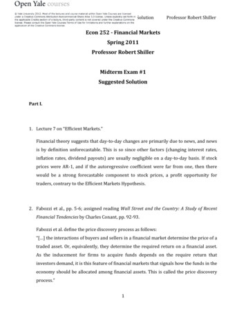
Econ 252 Spring 2011Midterm Exam #1 - SolutionQuestion 3Professor Robert Shiller(a) Making use of the fact that the Sharpe-ratio of the Tangency Portfolio is the slope of theTangency Line, one can compute the Sharpe-ratio of the Tangency Portfolio asSRTP µP 2 µP1 0.085 0.055 0.3.σ P 2 σ P10.25 0.15(b) As all portfolios on the Tangency Line have identical Sharpe-ratio, it follows thatportfolio 1 (as well as portfolio 2) have Sharpe-ratio 0.3. Then, it follows from theformula of the Sharpe-ratio that0.3 µP1 rf0.055 rf 0.3 ,σ P10.15implying that rf 0.01 1%.If the hint is used, one obtains0.25 µP1 rf0.055 rf 0.25 ,σ P10.15implying that rf 0.0175 1.75%.(c) The Sharpe-ratio of the Tangency Portfolio is equal toSRTP µTP rf0.06 0.02 SRTP 0.2.σ TP0.2With the risk-free rate of 2%, the maximum expected return that you can generategiven 25% return standard deviation corresponds to a portfolio on the secondTangency Line. Hence, the Sharpe-ratio of this portfolio equals 0.2. One thereforeobtains the maximum expected return as0.2 µP rfµ 0.02 0.2 P µP 0.07.σP0.25So, the maximum expected return is 7%.12

Econ 252 Spring 2011Midterm Exam #1 - SolutionProfessor Robert Shiller(d) In the context of the original tangency line, one can achieve 8.5% expected return for25% return standard deviation (which is exactly Portfolio 2). In the context of thesecond tangency line, one can only achieve 7% expected return for 25% returnstandard deviation. Therefore, the original tangency line is preferable.13

2. Fabozzi et al., pp. 5-6; assigned reading Wall Street and the Country: A Study of Recent Financial Tendencies by Charles . They make the data unreliable guides to the future, as there may have been no past . state that there are ways to modify the CAPM for fat tails. Econ 252 Spring 2011 Midterm Exam #1 - Solution Professor Robert .