WIXLIB

1.3 Depth Image Enhancement3values are used to estimate the phase-difference td as Q3 Q4td arctanQ1 Q2(1.1)where Q1 to Q4 represent the amount of electric charge for the control signals C1 toC4 respectively [37, 71, 67]. The corresponding distance d can then be calculated,using c the speed of light and f the signal frequency:d c td.2 f 2π(1.2)Here the quantity c/(2 f ) is the maximum distance that can be measured withoutambiguity, as will be explained in chapter 2.Fig. 1.2 Depth can be calculated by measuring the phase delay between radiated and reflected IRsignals. The quantities Q1 to Q4 represent the amount of electric charge for control signals C1 toC4 respectively.1.3 Depth Image EnhancementThis section describes the characteristic sources of error in ToF imaging. Somemethods for reducing these errors are discussed. The case of motion blur, whichis particularly problematic, is considered in detail.

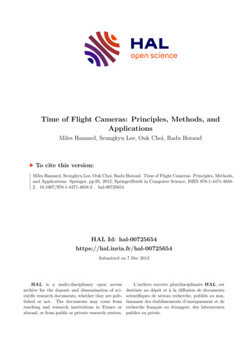
41 Characterization of Time-of-Flight Data1.3.1 Systematic Depth ErrorFrom the principle and architecture of ToF sensing, depth cameras suffer from several systematic errors such as IR demodulation error, integration time error, amplitude ambiguity and temperature error [37]. As shown in fig. 1.3 (a), longer integration increases signal to noise ratio, which, however, is also related to the frame rate.Figure 1.3 (b) shows that the amplitude of the reflected IR signal varies according tothe color of the target object as well as the distance from the camera. The ambiguityof IR amplitude introduces noise into the depth calculation.(a) Integration Time Error: Longer integration time shows higher depth accuracy (right) thanshorter integration time (left).(b) IR Amplitude Error: 3D points of the same depth (chessboard on the left) show different IRamplitudes (chessboard on the right) according to the color of the target object.Fig. 1.3 Systematic noise and error: These errors come from the ToF principle of depth measurement.

1.3 Depth Image Enhancement51.3.2 Non-Systematic Depth ErrorLight scattering [86] gives rise to artifacts in the depth image, due to the low sensitivity of the device. As shown in fig. 1.4 (a), close objects (causing IR saturation) inthe lower-right part of the depth image introduce depth distortion in other regions,as indicated by dashed circles. Multipath error [41] occurs when a depth calculation in a sensor pixel is an superposition of multiple reflected IR signals. This effectbecomes serious around the concave corner region as shown in fig. 1.4 (b). Objectboundary ambiguity [95] becomes serious when we want to reconstruct a 3D scenebased on the depth image. Depth pixels near boundaries fall in between foregroundand background, giving rise to 3D structure distortion.1.3.3 Motion BlurMotion blur, caused by camera or target object motions, is a critical error source foron-line 3D capturing and reconstruction with ToF cameras. Because the 3D depthmeasurement is used to reconstruct the 3D geometry of scene, blurred regions ina depth image lead to serious distortions in the subsequent 3D reconstruction. Inthis section, we study the theory of ToF depth sensors and analyze how motion bluroccurs, and what it looks like. Due the its unique sensing architecture, motion blurin the ToF depth camera is quite different from that of color cameras, which meansthat existing deblurring methods are inapplicable.The motion blur observed in a depth image has a different appearance from thatin a color image. Color motion blur shows smooth color transitions between foreground and background regions [109, 115, 121]. On the other hand, depth motionblur tends to present overshoot or undershoot in depth-transition regions. This isdue to the different sensing architecture in ToF cameras, as opposed to conventionalcolor cameras. The ToF depth camera emits an IR signal of a specific frequency, andmeasures the phase difference between the emitted and reflected IR signals to obtainthe depth from the camera to objects. While calculating the depth value from the IRmeasurements, we need to perform a non-linear transformation. Due to this architectural difference, the smooth error in phase measurement can cause uneven errorterms, such as overshoot or undershoot. As a result, such an architectural difference between depth and color cameras makes the previous color image deblurringalgorithms inapplicable to depth images.Special cases of this problem have been studied elsewhere. Hussmann et al. [61]introduce a motion blur detection technique on a conveyor belt, in the presence ofa single directional motion. Lottner et al. [79] propose an internal sensor controlsignal based blur detection method that is not appropriate in general settings. Lindner et al. [76] model the ToF motion blur in the depth image, to compensate forthe artifact. However, they introduce a simple blur case without considering the ToFprinciple of depth sensing. Lee et al. [73, 74] examine the principle of ToF depthblur artifacts, and propose systematic blur-detection and deblurring methods.

61 Characterization of Time-of-Flight Data(a) Light Scattering: IR saturation in the lower-right part of the depth image causes depthdistortion in other parts, as indicated by dashed circles.(b) Multipath Error: The region inside the concave corner is affected, and shows distorted depthmeasurements.(c) Object Boundary Ambiguity: Several depth points on an object boundary are located inbetween foreground and background, resulting in 3D structure distortion.Fig. 1.4 Non-systematic noise and error: Based on the depth-sensing principle, scene-structuremay cause characteristic errors.Based on the depth sensing principle, we will investigate how motion blur occurs, and what are its characteristics. Let’s assume that any motion from camera

1.3 Depth Image Enhancement7or object occurs during the integration time, which changes the phase difference ofthe reflected IR as indicated by the gray color in fig. 1.2. In order to collect enoughelectric charge Q1 to Q4 to calculate depth (1.1), we have to maintain a sufficientintegration time. According to the architecture type, integration time can vary, butthe integration time is the major portion of the processing time. Suppose that n cycles are used for the depth calculation. In general, we repeat the calculation n timesduring the integration time to increase the signal-to-noise ratio, and so nQ3 nQ4(1.3)td arctannQ1 nQ2where Q1 to Q4 represent the amount of electric charge for the control signals C1 toC4 respectively (cf. eqn. 1.1 and fig. 1.2). The depth calculation formulation 1.3 ex-Fig. 1.5 ToF depth motion-blur due to movement of the target object.pects that the reflected IR during the integration time comes from a single 3D pointof the scene. However, if there is any camera or object motion during the integrationtime, the calculated depth will be corrupted. Figure 1.5 shows an example of thissituation. The red dot represents a sensor pixel of the same location. Due the themotion of the chair, the red dot sees both foreground and background sequentiallywithin its integration time, causing a false depth calculation as shown in the thirdimage in fig. 1.5. The spatial collection of these false-depth points looks like bluraround moving object boundaries, where significant depth changes are present.Figure 1.6 illustrates what occurs at motion blur pixels in the ‘2-tab’ architecture,where only two electric charge values are available. In other words, only Q1 Q2and Q3 Q4 values are stored, instead of all separate Q values. Figure 1.6 (a) is thecase where no motion blur occurs. In the plot of Q1 Q2 versus Q3 Q4 in the thirdcolumn, all possible regular depth values are indicated by blue points, making adiamond shape. If there is a point deviating from it, as an example shown in fig. 1.6(b), it means that their is a problem in between the charge values Q1 to Q4 . As wealready explained in fig. 1.2, this happens when there exist multiple reflected signalswith different phase values. Let’s assume that a new reflected signal, of a differentphase value, comes in from the mth cycle out of a total of n cycles during the firsthalf or second half of the integration time. A new depth is then obtained as nQ̂3 nQ̂4(1.4)td (m) arctan(mQ1 (n m)Q̂1 ) (mQ2 (n m)Q̂2 )

81 Characterization of Time-of-Flight Data(a)(b)Fig. 1.6 ToF depth sensing and temporal integration.td (m) arctan (mQ3 (n m)Q̂3 ) (mQ4 (n m)Q̂4 )nQ̂1 nQ̂2 (1.5)in the first or second-half of the integration time, respectively. Using the depth calculation formulation (eq 1.1), we simulate all possible blur models. Figure 1.7 illustrates several examples of depth images taken by ToF cameras, having depth valuetransitions in motion blur regions. Actual depth values along the blue and red cuts ineach image are presented in the following plots. The motion blurs of depth images inthe middle show unusual peaks (blue cut) which cannot be observed in conventionalcolor motion blur. Figure 1.8 shows how motion blur appears in 2-tap case. In thesecond phase where control signals C3 and C4 collect electric charges, the reflectedIR signal is a mixture of background and foreground. Unlike color motion blurs,depth motion blurs often show overshoot or undershoot in their transition betweenforeground and background regions. This means that motion blurs result in higheror lower calculated depth than all near foreground and background depth values, asdemonstrated in fig. 1.9.In order to verify this characteristic situation, we further investigate the depthcalculation formulation in equation 1.5. Firstly we re-express equation 1.4 as nQ̂3 nQ̂4td (m) arctan(1.6)m(Q1 Q̂1 Q2 Q̂2 ) n(Q̂1 Q̂2 )

1.3 Depth Image Enhancement9Fig. 1.7 Sample depth value transitions from depth motion blur images captured by an SR4000T o F camera.Fig. 1.8 Depth motion blur in 2-tap case.The first derivative of the equation 1.6 is zero, meaning local maxima or local minima, under the following conditions:1td′ (m) 1 nQ̂3 nQ̂4m(Q1 Q̂1 Q2 Q̂2 ) n(Q̂1 Q̂2 ) 2(m(Q1 Q̂1 Q2 Q̂2 ) n(Q̂1 Q̂2 ))2 0(nQ̂3 nQ̂4 )2 (m(Q1 Q̂1 Q2 Q̂2 ) n(Q̂1 Q̂2 ))2(1.7)

101 Characterization of Time-of-Flight DataFig. 1.9 ToF depth motion blur simulation results.m nQ̂2 Q̂11 2Q̂1 nQ1 Q̂1 Q2 Q̂22Q1 2Q̂1(1.8)Fig. 1.10 Half of the all motion blur cases make local peaks.Figure 1.10 shows that statistically half of all cases have overshoots or undershoots. In a similar manner, the motion blur model of 1-tap (eqn. 1.9) and 4-tap(eqn. 1.10) cases can be derived. Because a single memory is assigned for recordingthe electric charge value of four control signals, the 1-tap case has four differentformulations upon each phase transition: nQ̂3 nQ̂4td (m) arctan(mQ1 (n m)Q̂1 ) nQ̂2 nQ̂3 nQ̂4td (m) arctannQ1 (mQ2 (n m)Q̂2 (mQ3 (n m)Q̂3 ) nQ̂4td (m) arctannQ̂1 nQ̂2 nQ3 (mQ4 (n m)Q̂4td (m) arctan(1.9)nQ̂1 nQ̂2On the other hand, the 4-tap case only requires a single formulation, which is:

1.3 Depth Image Enhancementtd (m) arctan 11(mQ3 (n m)Q̂3 ) (mQ4 (n m)Q̂4 )(mQ1 (n m)Q̂1 ) (mQ2 (n m)Q̂2 ) (1.10)Now, by investigating the relation between control signals, any corrupted depth easily can be identified. From the relation between Q1 and Q4 , we find the followingrelation:Q1 Q2 Q3 Q4 K.(1.11)Let’s call this the Plus Rule, where K is the total amount of charged electrons. Another relation is the following formulation, called the Minus Rule: Q1 Q2 Q3 Q4 K.(1.12)In fact, neither formulation exclusively represents motion blur. Any other event thatcan break the relation between the control signals, and can be detected by one ofthe rules, is an error which must be detected and corrected. We conclude that ToFmotion blur can be detected by one or more of these rules.(a) Depth images with motion blur(b) Intensity images with detected motion blur regions (indicated by white color)Fig. 1.11 Depth image motion blur detection results by the proposed method.Figure 1.11 (a) shows depth image samples with motion blur artifacts due to various object motions such as rigid body, multiple body and deforming body motionsrespectively. Motion blur occurs not just around object boundaries; inside an object,

121 Characterization of Time-of-Flight Dataany depth differences that are observed within the integration time will also causemotion blur. Figure 1.11 (b) shows detected motion blur regions indicated by whitecolor on respective depth and intensity images, by the method proposed in [73].This is very straightforward but effective and fast method, which is fit for hardwareimplementation without any additional frame memory or processing time.1.4 Evaluation of Time-of-Flight and Structured-Light DataThe enhancement of ToF and structured light (e.g. Kinect [106]) data is an importanttopic, owing to the physical limitations of these devices (as described in sec. 1.3).The characterization of depth-noise, in relation to the particular sensing architecture,is a major issue. This can be addressed using bilateral [118] or non-local [60] filters,or in wavelet-space [34], using prior knowledge of the spatial noise distribution.Temporal filtering [81] and video-based [28] methods have also been proposed.The upsampling of low resolution depth images is another critical issue. Oneapproach is to apply color super-resolution methods on ToF depth images directly[102]. Alternatively, a high resolution color image can be used as a reference fordepth super-resolution [117, 3]. The denoising and upsampling problems can alsobe addressed together [15], and in conjunction with high-resolution monocular [90]or binocular [27] color images.It is also important to consider the motion artifacts [79] and multipath [41] problems which are characteristic of ToF sensors. The related problem of ToF depthconfidence has been addressed using random-forest methods [95]. Other issues withT o F sensors include internal and external calibration [42, 77, 52], as well as rangeambiguity [18]. In the case of Kinect, a unified framework of dense depth data extraction and 3D reconstruction has been proposed [88].Despite the increasing interest in active depth-sensors, there are many unresolvedissues regarding the data produced by these devices, as outlined above. Furthermore,the lack of any standardized data sets, with ground truth, makes it difficult to makequantitative comparisons between different algorithms.The Middlebury stereo [99], multiview [103] and Stanford 3D scan [21] data sethave been used for the evaluation of depth image denoising, upsampling and 3Dreconstruction methods. However, these data sets do not provide real depth imagestaken by either ToF or structured-light depth sensors, and consist of illuminationcontrolled diffuse material objects. While previous depth accuracy enhancementmethods demonstrate their experimental results on their own data set, our understanding of the performance and limitations of existing algorithms will remain partial without any quantitative evaluation against a standard data set. This situationhinders the wider adoption and evolution of depth-sensor systems.In this section, we propose a performance evaluation framework for both ToFand structured-light depth images, based on carefully collected depth-maps and theirground truth images. First, we build a standard depth data set; calibrated depth images captured by a ToF depth camera and a structured light system. Ground truth

1.4 Evaluation of Time-of-Flight and Structured-Light Data13depth is acquired from a commercial 3D scanner. The data set spans a wide rangeof objects, organized according to geometric complexity (from smooth to rough), aswell as radiometric complexity (diffuse, specular, translucent and subsurface scattering). We analyze systematic and non-systematic error sources, including the accuracy and sensitivity with respect to material properties. We also compare the characteristics and performance of the two different types of depth sensors, based on extensive experiments and evaluations. Finally, to justify the usefulness of the data set,we use it to evaluate simple denoising, super-resolution and inpainting algorithms.1.4.1 Depth SensorsAs described in section 1.2, the ToF depth sensor emits IR waves to target objects,and measures the phase delay of reflected IR waves at each sensor pixel, to calculatethe distance travelled. According to the color, reflectivity and geometric structure ofthe target object, the reflected IR light shows amplitude and phase variations, causing depth errors. Moreover, the amount of IR is limited by the power consumptionof the device, and therefore the reflected IR suffers from low signal-to-noise ratio(SNR). To increase the SNR, ToF sensors bind multiple sensor pixels to calculate asingle depth pixel value, which decreases the effective image size. Structured lightdepth sensors project an IR pattern onto target objects, which provides a uniqueillumination code for each surface point observed at by a calibrated IR imaging sensor. Once the correspondence between IR projector and IR sensor is identified bystereo matching methods, the 3D position of each surface point can be calculated bytriangulation.In both sensor types, reflected IR is not a reliable cue for all surface materials.For example, specular materials cause mirror reflection, while translucent materialscause IR refraction. Global illumination also interferes with the IR sensing mechanism, because multiple reflections cannot be handled by either sensor type.1.4.2 Standard Depth Data SetA range of commercial ToF depth cameras have been launched in the market, suchas PMD, PrimeSense, Fotonic, ZCam, SwissRanger, 3D MLI, and others. Kinectis the first widely successful commercial product to adopt the IR structured lightprinciple. Among many possibilities, we specifically investigate two depth cameras:a ToF type SR4000 from MESA Imaging [80], and a structured light type MicrosoftKinect [105]. We select these two cameras to represent eac

Applications Miles Hansard, Seungkyu Lee, Ouk Choi, Radu Horaud To cite this version: Miles Hansard, Seungkyu Lee, Ouk Choi, Radu Horaud. Time of Flight Cameras: Principles, Methods, and Applications. Springer, pp.95, 2012, SpringerBriefs in Computer Science, ISBN 978-1-4471-4658-2. 10.1007/978-1-4471-4658-2 . hal-00725654