Transcription
Chapter 3Electric Potential3.1 Potential and Potential Energy. 3-23.2 Electric Potential in a Uniform Field. 3-53.3 Electric Potential due to Point Charges . 3-63.3.1 Potential Energy in a System of Charges. 3-83.4 Continuous Charge Distribution . 3-93.5 Deriving Electric Field from the Electric Potential . 3-103.5.1 Gradient and Equipotentials. 3-11Example 3.1: Uniformly Charged Rod . 3-13Example 3.2: Uniformly Charged Ring . 3-15Example 3.3: Uniformly Charged Disk . 3-16Example 3.4: Calculating Electric Field from Electric Potential. 3-183.6 Summary. 3-183.7 Problem-Solving Strategy: Calculating Electric Potential. 3-203.8 Solved Problems . 3-223.8.13.8.23.8.33.8.4Electric Potential Due to a System of Two Charges. 3-22Electric Dipole Potential . 3-23Electric Potential of an Annulus . 3-24Charge Moving Near a Charged Wire . 3-253.9 Conceptual Questions . 3-263.10 Additional Problems . 3-273.10.1 Cube . 3-273.10.2 Three Charges . 3-273.10.3 Work Done on Charges. 3-273.10.4 Calculating E from V . 3-283.10.5 Electric Potential of a Rod . 3-283.10.6 Electric Potential. 3-293.10.7 Calculating Electric Field from the Electric Potential . 3-293.10.8 Electric Potential and Electric Potential Energy. 3-303.10.9. Electric Field, Potential and Energy . 3-303-1
Electric Potential3.1 Potential and Potential EnergyIn the introductory mechanics course, we have seen that gravitational force from theEarth on a particle of mass m located at a distance r from Earth’s center has an inversesquare form:Fg GMmrˆr2(3.1.1)where G 6.67 10 11 N m 2 /kg 2 is the gravitational constant and r̂ is a unit vectorpointing radially outward. The Earth is assumed to be a uniform sphere of mass M. Thecorresponding gravitational field g , defined as the gravitational force per unit mass, isgiven byg Fgm GMrˆr2(3.1.2)Notice that g only depends on M, the mass which creates the field, and r, the distancefrom M.Figure 3.1.1Consider moving a particle of mass m under the influence of gravity (Figure 3.1.1). Thework done by gravity in moving m from A to B is GMmGMmWg Fg d s 2 dr rA r rBr rBrA 1 1 GMm rB rA (3.1.3)The result shows that Wg is independent of the path taken; it depends only on theendpoints A and B. It is important to draw distinction between Wg , the work done by the3-2
field and Wext , the work done by an external agent such as you. They simply differ by anegative sign: Wg Wext .Near Earth’s surface, the gravitational field g is approximately constant, with amagnitude g GM / rE 2 9.8 m/s 2 , where rE is the radius of Earth. The work done bygravity in moving an object from height y A to yB (Figure 3.1.2) isBByBAAyAWg Fg d s mg cos θ ds mg cos φ ds mg dy mg ( yB y A )(3.1.4)Figure 3.1.2 Moving a mass m from A to B.The result again is independent of the path, and is only a function of the change invertical height yB y A .In the examples above, if the path forms a closed loop, so that the object moves aroundand then returns to where it starts off, the net work done by the gravitational field wouldbe zero, and we say that the gravitational force is conservative. More generally, a force Fis said to be conservative if its line integral around a closed loop vanishes:v G GF d s 0(3.1.5)When dealing with a conservative force, it is often convenient to introduce the concept ofpotential energy U. The change in potential energy associated with a conservative forceF acting on an object as it moves from A to B is defined as:B U U B U A F d s WA(3.1.6)where W is the work done by the force on the object. In the case of gravity, W Wg andfrom Eq. (3.1.3), the potential energy can be written asUg GMm U0r(3.1.7)3-3
where U 0 is an arbitrary constant which depends on a reference point. It is oftenconvenient to choose a reference point where U 0 is equal to zero. In the gravitationalcase, we choose infinity to be the reference point, with U 0 (r ) 0 . Since U g dependson the reference point chosen, it is only the potential energy difference U g that hasphysical importance. Near Earth’s surface where the gravitational field g isapproximately constant, as an object moves from the ground to a height h, the change inpotential energy is U g mgh , and the work done by gravity is Wg mgh .A concept which is closely related to potential energy is “potential.” From U , thegravitational potential can be obtained as Vg U gmBBAA (Fg / m) d s g d s(3.1.8)Physically Vg represents the negative of the work done per unit mass by gravity tomove a particle from A to B .Our treatment of electrostatics is remarkably similar to gravitation. The electrostatic forceJGF e given by Coulomb’s law also has an inverse-square form. In addition, it is alsoconservative. In the presence of an electric field E , in analogy to the gravitational fieldg , we define the electric potential difference between two points A and B asBBAA V (Fe / q0 ) d s E d s(3.1.9)where q0 is a test charge. The potential difference V represents the amount of workdone per unit charge to move a test charge q0 from point A to B, without changing itskinetic energy. Again, electric potential should not be confused with electric potentialenergy. The two quantities are related by U q0 V(3.1.10)The SI unit of electric potential is volt (V):1volt 1 joule/coulomb (1 V 1 J/C)(3.1.11)When dealing with systems at the atomic or molecular scale, a joule (J) often turns out tobe too large as an energy unit. A more useful scale is electron volt (eV), which is definedas the energy an electron acquires (or loses) when moving through a potential differenceof one volt:3-4
1eV (1.6 10 19 C)(1V) 1.6 10 19 J(3.1.12)3.2 Electric Potential in a Uniform FieldConsider a charge q moving in the direction of a uniform electric field E E0 ( ˆj) , asshown in Figure 3.2.1(a).(b)(a)Figure 3.2.1 (a) A charge q which moves in the direction of a constant electric field E .(b) A mass m that moves in the direction of a constant gravitational field g .Since the path taken is parallel to E , the potential difference between points A and B isgiven byBBAA V VB VA E d s E0 ds E0 d 0(3.2.1)implying that point B is at a lower potential compared to A. In fact, electric field linesalways point from higher potential to lower. The change in potential energy is U U B U A qE0 d . Since q 0, we have U 0 , which implies that the potentialenergy of a positive charge decreases as it moves along the direction of the electric field.The corresponding gravitational analogy, depicted in Figure 3.2.1(b), is that a mass mloses potential energy ( U mg d ) as it moves in the direction of the gravitationalfield g .Figure 3.2.2 Potential difference due to a uniform electric fieldWhat happens if the path from A to B is not parallel to E , but instead at an angle θ, asshown in Figure 3.2.2? In that case, the potential difference becomes3-5
B V VB VA E d s E s E0 s cos θ E0 yA(3.2.2)Note that y increase downward in Figure 3.2.2. Here we see once more that moving alongthe direction of the electric field E leads to a lower electric potential. What would thechange in potential be if the path were A C B ? In this case, the potential differenceconsists of two contributions, one for each segment of the path: V VCA VBC(3.2.3)When moving from A to C, the change in potential is VCA E0 y . On the other hand,when going from C to B, VBC 0 since the path is perpendicular to the direction of E .Thus, the same result is obtained irrespective of the path taken, consistent with the factthat E is conservative.Notice that for the path A C B , work is done by the field only along the segmentAC which is parallel to the field lines. Points B and C are at the same electric potential,i.e., VB VC . Since U q V , this means that no work is required in moving a chargefrom B to C. In fact, all points along the straight line connecting B and C are on the same“equipotential line.” A more complete discussion of equipotential will be given inSection 3.5.3.3 Electric Potential due to Point ChargesNext, let’s compute the potential difference between two points A and B due to a charge Q. The electric field produced by Q is E (Q / 4πε 0 r 2 )rˆ , where r̂ is a unit vectorpointing toward the field point.Figure 3.3.1 Potential difference between two points due to a point charge Q.From Figure 3.3.1, we see that rˆ d s ds cos θ dr , which gives V VB VA BAQ4πε 0 r2rˆ d s BAQ4πε 0 r2dr Q 1 1 4πε 0 rB rA (3.3.1)3-6
Once again, the potential difference V depends only on the endpoints, independent ofthe choice of path taken.As in the case of gravity, only the difference in electrical potential is physicallymeaningful, and one may choose a reference point and set the potential there to be zero.In practice, it is often convenient to choose the reference point to be at infinity, so that theelectric potential at a point P becomesPVP E d s(3.3.2) With this reference, the electric potential at a distance r away from a point charge QbecomesQ4πε 0 r1V (r ) (3.3.3)When more than one point charge is present, by applying the superposition principle, thetotal electric potential is simply the sum of potentials due to individual charges:V (r ) 14πε 0qi rii ke iqiri(3.3.4)A summary of comparison between gravitation and electrostatics is tabulated below:GravitationElectrostaticsMass mCharge qGravitational force Fg GMmrˆr2Gravitational field g Fg / mBPotential energy change U Fg d sABGravitational potential Vg g d sAFor a source M: Vg GMr U g mg d (constant g )Coulomb force Fe keQqrˆr2Electric field E Fe / qBPotential energy change U Fe d sABElectric Potential V E d sAFor a source Q: V keQr U qEd (constant E )3-7
3.3.1 Potential Energy in a System of ChargesIf a system of charges is assembled by an external agent, then U W Wext . That is,the change in potential energy of the system is the work that must be put in by an externalagent to assemble the configuration. A simple example is lifting a mass m through aheight h. The work done by an external agent you, is mgh (The gravitational fielddoes work mgh ). The charges are brought in from infinity without acceleration i.e. theyare at rest at the end of the process. Let’s start with just two charges q1 and q2 . Let thepotential due to q1 at a point P be V1 (Figure 3.3.2).Figure 3.3.2 Two point charges separated by a distance r12 .The work W2 done by an agent in bringing the second charge q2 from infinity to P isthen W2 q2V1 . (No work is required to set up the first charge and W1 0 ). SinceV1 q1 / 4πε 0 r12 , where r12 is the distance measured from q1 to P, we haveU12 W2 q1q24πε 0 r121(3.3.5)If q1 and q2 have the same sign, positive work must be done to overcome the electrostaticrepulsion and the potential energy of the system is positive, U12 0 . On the other hand, ifthe signs are opposite, then U12 0 due to the attractive force between the charges.Figure 3.3.3 A system of three point charges.To add a third charge q3 to the system (Figure 3.3.3), the work required is3-8
W3 q3 ( V1 V2 ) q3 q1 q2 4πε 0 r13 r23 (3.3.6)The potential energy of this configuration is thenU W2 W3 1 q1q2 q1q3 q2 q3 r13r234πε 0 r12 U12 U13 U 23 (3.3.7)The equation shows that the total potential energy is simply the sum of the contributionsfrom distinct pairs. Generalizing to a system of N charges, we haveU 14πε 0NN i 1 j 1j iqi q jrij(3.3.8)where the constraint j i is placed to avoid double counting each pair. Alternatively,one may count each pair twice and divide the result by 2. This leads toU 18πε 0NN i 1 j 1j iqi q jrij 1 N 1 qi2 i 1 4πε 0 qj 1 NqiV (ri ) 2 j 1 rij i 1j i N(3.3.9)where V (ri ) , the quantity in the parenthesis, is the potential at ri (location of qi) due to allthe other charges.3.4 Continuous Charge DistributionIf the charge distribution is continuous, the potential at a point P can be found bysumming over the contributions from individual differential elements of charge dq .Figure 3.4.1 Continuous charge distribution3-9
Consider the charge distribution shown in Figure 3.4.1. Taking infinity as our referencepoint with zero potential, the electric potential at P due to dq isdV dq4πε 0 r1(3.4.1)Summing over contributions from all differential elements, we haveV 14πε 0 dqr(3.4.2)3.5 Deriving Electric Field from the Electric PotentialIn Eq. (3.1.9) we established the relation between E and V. If we consider two pointswhich are separated by a small distance d s , the following differential form is obtained:dV E d s(3.5.1)In Cartesian coordinates, E Ex ˆi E y ˆj Ez kˆ and d s dx ˆi dyˆj dz kˆ , we have()()dV Ex ˆi E y ˆj Ez kˆ dx ˆi dyˆj dz kˆ Ex dx E y dy Ez dz(3.5.2)which impliesEx V V V, Ey , Ez x y z(3.5.3)By introducing a differential quantity called the “del (gradient) operator” ˆ ˆ ˆi j k x y z(3.5.4)the electric field can be written as V ˆ V ˆ V ˆ ˆ ˆ ˆ E Ex ˆi E y ˆj Ez kˆ i j k i j k V V y z y z x xE V(3.5.5)Notice that operates on a scalar quantity (electric potential) and results in a vectorquantity (electric field). Mathematically, we can think of E as the negative of thegradient of the electric potential V . Physically, the negative sign implies that if3-10
V increases as a positive charge moves along some direction, say x, with V / x 0 ,then there is a non-vanishing component of E in the opposite direction ( Ex 0) . In thecase of gravity, if the gravitational potential increases when a mass is lifted a distance h,the gravitational force must be downward.If the charge distribution possesses spherical symmetry, then the resulting electric field isa function of the radial distance r, i.e., E Er rˆ . In this case, dV Er dr. If V (r ) isknown, then E may be obtained as dV E Er rˆ r̂ dr (3.5.6)For example, the electric potential due to a point charge q is V (r ) q / 4πε 0 r . Using theabove formula, the electric field is simply E (q / 4πε 0 r 2 )rˆ .3.5.1 Gradient and EquipotentialsSuppose a system in two dimensions has an electric potential V ( x, y ) . The curvescharacterized by constant V ( x, y ) are called equipotential curves. Examples ofequipotential curves are depicted in Figure 3.5.1 below.Figure 3.5.1 Equipotential curvesIn three dimensions we have equipotential surfaces and they are described byV ( x, y, z ) constant. Since E V , we can show that the direction of E is alwaysperpendicular to the equipotential through the point. Below we give a proof in twodimensions. Generalization to three dimensions is straightforward.Proof:Referring to Figure 3.5.2, let the potential at a point P ( x, y ) be V ( x, y ) . How much isV changed at a neighboring point P( x dx, y dy) ? Let the difference be written as3-11
dV V ( x dx, y dy ) V ( x, y ) V Vdx dy V ( x, y ) x y V V V ( x, y ) x dx y dy (3.5.7)Figure 3.5.2 Change in V when moving from one equipotential curve to anotherWith the displacement vector given by d s dx ˆi dy ĵ , we can rewrite dV as V ˆ VdV i y xˆj dx ˆi dyˆj ( V ) d s E d s ()(3.5.8)If the displacement d s is along the tangent to the equipotential curve through P(x,y),then dV 0 because V is constant everywhere on the curve. This implies that E d salong the equipotential curve. That is, E is perpendicular to the equipotential. In Figure3.5.3 we illustrate some examples of equipotential curves. In three dimensions theybecome equipotential surfaces. From Eq. (3.5.8), we also see that the change in potentialdV attains a maximum when the gradient V is parallel to d s : dV max V ds (3.5.9)Physically, this means that V always points in the direction of maximum rate of changeof V with respect to the displacement s.Figure 3.5.3 Equipotential curves and electric field lines for (a) a constant E field, (b) apoint charge, and (c) an electric dipole.3-12
The properties of equipotential surfaces can be summarized as follows:(i)The electric field lines are perpendicular to the equipotentials and point fromhigher to lower potentials.(ii)By symmetry, the equipotential surfaces produced by a point charge form a familyof concentric spheres, and for constant electric field, a family of planesperpendicular to the field lines.(iii) The tangential component of the electric field along the equipotential surface iszero, otherwise non-vanishing work would be done to move a charge from onepoint on the surface to the other.(iv) No work is required to move a particle along an equipotential surface.A useful analogy for equipotential curves is a topographic map (Figure 3.5.4). Eachcontour line on the map represents a fixed elevation above sea level. Mathematically it isexpressed as z f ( x, y ) constant . Since the gravitational potential near the surface ofEarth is Vg gz , these curves correspond to gravitational equipotentials.Figure 3.5.4 A topographic mapExample 3.1: Uniformly Charged RodConsider a non-conducting rod of length having a uniform charge density λ . Find theelectric potential at P , a perpendicular distance y above the midpoint of the rod.Figure 3.5.5 A non-conducting rod of lengthand uniform charge density λ .3-13
Solution:Consider a differential element of length dx′ which carries a charge dq λ dx′ , as shownin Figure 3.5.5. The source element is located at ( x′, 0) , while the field point P is locatedon the y-axis at (0, y ) . The distance from dx′ to P is r ( x′2 y 2 )1/ 2 . Its contribution tothe potential is given bydq1λ dx′ 4πε 0 r4πε 0 ( x′2 y 2 )1/ 21dV Taking V to be zero at infinity, the total potential due to the entire rod isV λ4πε 0 /2 /2dx′x ′2 y 2 λln x′ x′2 y 2 4πε 0 ( / 2) ( / 2) 2 y 2λ ln 4πε 0 ( / 2) ( / 2) 2 y 2 /2 /2(3.5.10)where we have used the integration formula dx′x′ y22( ln x′ x′2 y 2A plot of V ( y ) / V0 , where V0 λ / 4πε 0 , as a function of y /)is shown in Figure 3.5.6Figure 3.5.6 Electric potential along the axis that passes through the midpoint of a nonconducting rod.In the limit y, the potential becomes3-14
( / 2) / 2 1 (2 y / ) 2 1 1 (2 y / ) 2λλln ln V 4πε 0 ( / 2) / 2 1 (2 y / ) 2 4πε 0 1 1 (2 y / ) 2 λ2ln 24πε 0 2 y / λln 2πε 0 y 2 2 λln 2 4πε 0 y (3.5.11)The corresponding electric field can be obtained asEy Vλ/2 y 2πε 0 y ( / 2) 2 y 2in complete agreement with the result obtained in Eq. (2.10.9).Example 3.2: Uniformly Charged RingConsider a uniformly charged ring of radius R and charge density λ (Figure 3.5.7). Whatis the electric potential at a distance z from the central axis?Figure 3.5.7 A non-conducting ring of radius R with uniform charge density λ .Solution:Consider a small differential element d R dφ ′ on the ring. The element carries acharge dq λ d λ R dφ ′ , and its contribution to the electric potential at P isdV dq1 λ R dφ ′ 4πε 0 r4πε 0 R 2 z 21The electric potential at P due to the entire ring is3-15
V dV λR14πε 02πλ R1R2 z 2 dφ ′ 4πεR2 z 20 14πε 0QR2 z 2(3.5.12)where we have substituted Q 2π Rλ for the total charge on the ring. In the limit zthe potential approaches its “point-charge” limit:V R,1 Q4πε 0 zFrom Eq. (3.5.12), the z-component of the electric field may be obtained asEz V 1 z z 4πε 0 1Qz 22 3/ 2R z 4πε 0 ( R z )Q22(3.5.13)in agreement with Eq. (2.10.14).Example 3.3: Uniformly Charged DiskConsider a uniformly charged disk of radius R and charge density σ lying in the xyplane. What is the electric potential at a distance z from the central axis?Figure 3.4.3 A non-conducting disk of radius R and uniform charge density σ.Solution:Consider a circular ring of radius r ′ and width dr ′ . The charge on the ring isdq′ σ dA′ σ (2π r ′dr ′). The field point P is located along the z -axis a distance zfrom the plane of the disk. From the figure, we also see that the distance from a point onthe ring to P is r (r ′2 z 2 )1/ 2 . Therefore, the contribution to the electric potential at PisdV dq1 σ (2π r ′dr ′) 4πε 0 r4πε 0 r ′2 z 213-16
By summing over all the rings that make up the disk, we haveV In the limit z σ4πε 0 R2π r ′dr ′r ′2 z 20 σ 2 2 r′ z 2ε 0 R 0σ 2 2R z z 2ε 0 (3.5.14)R,1/ 2 R2 R z z 1 2 z 22 R2 z 1 2 2z , and the potential simplifies to the point-charge limit:V σ R21 σ (π R 2 )1 Q 2ε 0 2 z 4πε 0 z 4πε 0 z As expected, at large distance, the potential due to a non-conducting charged disk is thesame as that of a point charge Q. A comparison of the electric potentials of the disk and apoint charge is shown in Figure 3.4.4.Figure 3.4.4 Comparison of the electric potentials of a non-conducting disk and a pointcharge. The electric potential is measured in terms of V0 Q / 4πε 0 R .Note that the electric potential at the center of the disk ( z 0 ) is finite, and its value isVc σRQR1 2Q 2V022ε 0 π R 2ε 0 4πε 0 R(3.5.15)This is the amount of work that needs to be done to bring a unit charge from infinity andplace it at the center of the disk.The corresponding electric field at P can be obtained as:Ez Vσ z 2ε 0 z z R2 z 2 z (3.5.16)3-17
which agrees with Eq. (2.10.18). In the limit R z , the above equation becomesEz σ / 2ε 0 , which is the electric field for an infinitely large non-conducting sheet.Example 3.4: Calculating Electric Field from Electric PotentialSuppose the electric potential due to a certain charge distribution can be written inCartesian Coordinates asV ( x, y, z ) Ax 2 y 2 Bxyzwhere A , B and C are constants. What is the associated electric field?Solution:The electric field can be found by using Eq. (3.5.3): V 2 Axy 2 Byz x VEy 2 Ax 2 y Bxz y VEz Bxy zEx Therefore, the electric field is E ( 2 Axy 2 Byz ) ˆi (2 Ax 2 y Bxz ) ˆj Bxy kˆ .3.6 Summary A force F is conservative if the line integral of the force around a closed loopvanishes: F d s 0 The change in potential energy associated with a conservative force F acting on anobject as it moves from A to B isB U U B U A F d sA3-18
The electric potential difference V between points A and B in an electric field E isgiven by V VB VA B U E dsAq0The quantity represents the amount of work done per unit charge to move a testcharge q0 from point A to B, without changing its kinetic energy. The electric potential due to a point charge Q at a distance r away from the charge isV 1 Q4πε 0 rFor a collection of charges, using the superposition principle, the electric potential isV 4πε 0Qi riiThe potential energy associated with two point charges q1 and q2 separated by adistance r12 isU 11 q1q24πε 0 r12From the electric potential V , the electric field may be obtained by taking thegradient of V :E VIn Cartesian coordinates, the components may be written asEx V V V, Ey , Ez x y zThe electric potential due to a continuous charge distribution isV 14πε 0 dqr3-19
3.7 Problem-Solving Strategy: Calculating Electric PotentialIn this chapter, we showed how electric potential can be calculated for both the discreteand continuous charge distributions. Unlike electric field, electric potential is a scalarquantity. For the discrete distribution, we apply the superposition principle and sum overindividual contributions:V ke iqiriFor the continuous distribution, we must evaluate the integralV ke dqrIn analogy to the case of computing the electric field, we use the following steps tocomplete the integration:(1) Start with dV kedq.r(2) Rewrite the charge element dq as λ dl dq σ dA ρ dV (length)(area)(volume)depending on whether the charge is distributed over a length, an area, or a volume.(3) Substitute dq into the expression for dV .(4) Specify an appropriate coordinate system and express the differential element (dl, dAor dV ) and r in terms of the coordinates (see Table 2.1.)(5) Rewrite dV in terms of the integration variable.(6) Complete the integration to obtain V.Using the result obtained for V , one may calculate the electric field by E V .Furthermore, the accuracy of the result can be readily checked by choosing a point Pwhich lies sufficiently far away from the charge distribution. In this limit, if the chargedistribution is of finite extent, the field should behave as if the distribution were a pointcharge, and falls off as 1/ r 2 .3-20
Below we illustrate how the above methodologies can be employed to compute theelectric potential for a line of charge, a ring of charge and a uniformly charged disk.Charged RodCharged RingCharged diskdq λ dx′dq λ dldq σ dAFigure(2) Express dq interms of chargedensity(3) Substitute dqinto expression fordV(4) Rewrite r and thedifferential elementin terms of theappropriatecoordinatesV (6) Integrate to get VDerive E from VPoint-chargefor ElimitdV kerλ dldV kerσ dArdx′dl R dφ ′dA 2π r ′ dr ′r x′ 2 y 2r R2 z 2r r ′2 z 2dV ke(5) Rewrite dVλ dx′dV keλ4πε0 /2/2λ dx′2 1/ 2V kedx′x′2 y2 ( / 2) ( / 2)2 y2λln 4πε0 ( / 2) ( / 2)2 y2 Ey V yλ/2 2πε 0 y ( / 2) 2 y 2Ey dV ke( x′ y )2ke Qy2y ke keEz Ez λ R dφ ′(R z )22 1/ 2Rλ( R z 2 )1/ 2(2π Rλ )2 dφ ′R zkeQz V z ( R 2 z 2 )3/ 2ke Qz2zRR0 22πσ r ′ dr ′(r ′2 z 2 )1/ 2V ke 2πσ 2keπσR2 z 2Q2dV keEz (r′ dr′(r′ z2 )1/22)z2 R2 z )(2keQ 2 2z R z R2 V 2keQ zz 2 zR z z 2 R2 Ez ke Qz2zR3-21
3.8 Solved Problems3.8.1 Electric Potential Due to a System of Two ChargesConsider a system of two charges shown in Figure 3.8.1.Figure 3.8.1 Electric dipoleFind the electric potential at an arbitrary point on the x axis and make a plot.Solution:The electric potential can be found by the superposition principle. At a point on the xaxis, we haveV ( x) qq 11 ( q)1 4πε 0 x a 4πε 0 x a 4πε 0 x a x a 1The above expression may be rewritten asV ( x)11 V0 x / a 1 x / a 1 where V0 q / 4πε 0 a . The plot of the dimensionless electric potential as a function of x/a.is depicted in Figure 3.8.2.Figure 3.8.23-22
As can be seen from the graph, V ( x) diverges at x / a 1 , where the charges arelocated.3.8.2 Electric Dipole PotentialConsider an electric dipole along the y-axis, as shown in the Figure 3.8.3. Find theelectric potential V at a point P in the x-y plane, and use V to derive the correspondingelectric field.Figure 3.8.3By superposition principle, the potential at P is given byV Vi i1 q q 4πε 0 r r where r 2 r 2 a 2 2ra cos θ . If we take the limit where ra, then 1/ 21 11 1 1 (a / r ) 2 2(a / r ) cos θ 1 (a / r ) 2 (a / r ) cos θ r rr 2 and the dipole potential can be approximated as1 11 (a / r ) 2 (a / r ) cos θ 1 (a / r ) 2 (a / r ) cos θ 4πε 0 r 22p rˆ2a cos θ p cos θq 24πε 0 r4πε 0 r4πε 0 r 2rV q where p 2aq ˆj is the electric dipole moment. In spherical polar coordinates, the gradientoperator is 1 ˆ1 rˆ θ φˆr θr sin θ φ r3-23
Since the potential is now a function of both r and θ , the electric field will havecomponents along the r̂ and θ̂ directions. Using E V , we haveEr V p cos θ1 V p sin θ , Eθ , Eφ 03 r 2πε 0 rr θ 4πε 0 r 33.8.3 Electric Potential of an AnnulusConsider an annulus of uniform charge density σ , as shown in Figure 3.8.4. Find theelectric potential at a point P along the symmetric axis.Figure 3.8.4 An annulus of uniform charge density.Solution:Consider a small differential element dA at a distance r away from point
3.3 Electric Potential due to Point Charges Next, let's compute the potential difference between two points A and B due to a charge Q. The electric field produced by Q is 2 0 E (/Q4πεr)ˆ JG, where is a unit vector pointing toward the field point. rˆ Figure 3.3.1 Potential difference between two points due to a point charge Q.