Transcription
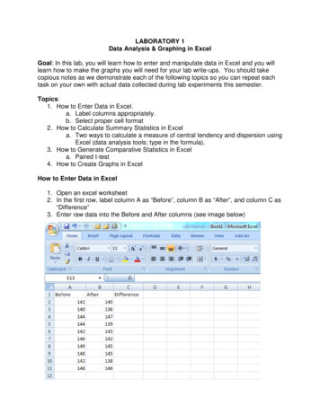
LABORATORY 1Data Analysis & Graphing in ExcelGoal: In this lab, you will learn how to enter and manipulate data in Excel and you willlearn how to make the graphs you will need for your lab write-ups. You should takecopious notes as we demonstrate each of the following topics so you can repeat eachtask on your own with actual data collected during lab experiments this semester.Topics:1. How to Enter Data in Excel.a. Label columns appropriately.b. Select proper cell format2. How to Calculate Summary Statistics in Excela. Two ways to calculate a measure of central tendency and dispersion usingExcel (data analysis tools; type in the formula).3. How to Generate Comparative Statistics in Excela. Paired t-test4. How to Create Graphs in ExcelHow to Enter Data in Excel1. Open an excel worksheet2. In the first row, label column A as “Before”, column B as “After”, and column C as“Difference”3. Enter raw data into the Before and After columns (see image below)
4. In the “Difference” column, enter a function (aka an equation or formula) to tellExcel to subtract the before values from the after values.a. Always start a formula with a “ ” symbol, then select the cell from column B,then type a “-“ symbol, then select the cell from column A, then hit enter.b. The result will be displayed when you hit the enter key (see “-2” and “-4”shown in cells C2 and C3 below). The formula is shown in cell C4.c. Once you type in the formula, you can copy and paste that formula into theremaining cells of column C.d. If you want to calculate a paired t-test by hand, you will need these differencevalues. Otherwise, you will not use them to make your graphs or analyses.
How to Calculate Summary Statistics in Excel: Two Methods1. Use the data analysis tools.a. Open the worksheet with your data. Select the “Data” tab, then “DataAnalysis” , then from the list choose “Descriptive Statistics”and select“OK”.b. From here, with your cursor in the Input Range , select your data in columnA. Then put your cursor in the Output Range blockand select an emptycell in your work sheet. Click the box labeled “Summary Statistics” so acheck mark appears, then select “OK” .
c. Excel will now show you the summary statistics. I have added highlights toshow the mean, standard deviation, standard error, and sample size whichare the summary statistics that you will most commonly use for your write-upsin our labs.
OR2. Type in the formulas. For any formula, you can then copy/paste into cells foradjacent columns (be sure to check that excel is using the correct cells to calculatethe values)a. Mean: the formula to tell Excel to calculate a mean is “ average(select cellshere)”. Type this formula into the appropriate cell and then hit enter.b. Standard Deviation: the formula to tell Excel to calculate a standard deviationis “ stdev(select cells here)” . Type this formula into the appropriate cell andthen hit enter.c. Sample size: the formula to tell Excel to calculate your sample size is“ count(select cells here)” . Type this formula into the appropriate cell andthen hit enter.d. Standard Error: The standard error is the standard deviation divided by thesquare root of the sample size. Therefore, the formula to tell Excel tocalculate a standard error is “ [select the cell for standard deviation]/sqrt([cellfor sample size])”. Type this formula into the appropriate cell and then hitenter.
How to Generate Comparative Statistics in Excel1. Use the data analysis tools.a. Open the worksheet with your data. Select the “Data” tab, then “DataAnalysis” , then choose “t-test: Paired Two Sample for Means”andselect “OK”.b. Next, you need to tell Excel which data to compare. To do this, click in theempty “Variable 1 Range” box and then click hold drag your Before data .Repeat this process with your “After” data for the “Variable 2 Range” . Thenclick the “Output Range” option , and then select an empty cell where excelwill begin to put your statistical output (NOTE: select a cell where theoutput will not overwrite existing data in your spreadsheet). Click “OK” .
c. Notice that the output from Excel includes a lot of information (note that themean is shown again here). For our purposes, you only need to include threepieces of information when you report your paired t-test results.i. You should include your degrees of freedom (for a paired T-test, this isthe sample size minus one) .ii. You should include your t statistic .iii. You should include your two-tailed P-value . NOTE: If a P-value isless than 0.05, then you know that your two groups that you comparedare significantly different from each other. If the P-value is greater thanor equal to 0.05, then the two groups are not different from each other.iv. Example of a sentence to be written in your results section:“Average heart rate decreased after frog hearts were exposed topilocarpine (t 2.98, df 9, P 0.016; Figure 1)”, where Figure onewould show your descriptive statistics (mean and error bars that aresome measure of dispersion).d. Hint: there is some information that you should NOT include in yourpapers:i. NO RAW DATA should be in your paper as either a table or graph.ii. DO NOT copy and paste the output shown above from Excel into yourlab write-up.
How to Create Graphs in Excel1. Plot the means.a. In this example, you willplot frog heart rate beforeand after treatment withtwo drugs (epinephrine,nicotine). First, calculateyour descriptive statisticsby one of the methodsshown above andorganize your resultsbelow the columns of dataas shown .b. Holding the CTRL buttonon your keyboard, selectthe “Before” value forepinephrine and thenfor nicotine .c. Select the “Insert” tab ,then Column , thenUnder 2D columns, selectthe first option. Whenyou click this option,you will see the image below.d. Note that “Series 1” is your “Before” values (we’ll re-name this in a minute).
e. Now we need to add the “After” values in a second “series”. To do this, besure to click the chart which will activate the “Chart Tools” area. In this area,select the “Design”tab, then “Select Data” , then “Add” .f. For series name, type “After” . Note that a nonsense characterautomatically occurs for the Series values . Delete this. With your cursor inthis box, hold the CTRL key and then select the after values for Heart Ratefor Epinephrine (cell C24) and Nicotine (cell G24). Click “OK” here and onthe next screen.
g. We usually want the y-axis to go to zero when presenting data. To do this,right click on your y-axis and select “Format Axis”. Select “AxisOptions” “Minimum” “Fixed” and then enter a “0”. Click “Close”.h. Now you will see the basic graph (image not shown). Next, you can fix thelabeling.2. Label the grapha. First, let’s fix the series 1 name and the names of the components of theseries.b. Click on the graph to bring up the Chart Tools tab. Select Design SelectData Series 1 Edit (on the Legend Entries side of the box). Then type in“Before” for the series name and click “OK”.c. Click on the graph to bring up the Chart Tools tab. Select Design SelectData Series 1 Edit (on the Horizontal Axes Legend side of the box). Thentype in “Epinephrine,Nicotine”, with the labels separated by a comma and nospace after the comma (otherwise your label will be moved over a spacewhen placed on your axis). Click “OK”, then click “OK” again. Now your graphhas the data labeled correctly and you need only to add labels to your axes.d. To label the x-axis, click on the graph to bring up the Chart Tools tab. SelectLayout Axis Titles Primary Horizontal Axis Title Below Axis. Now atitle will appear at the x-axis on your graph; click in the text box and type yourtitle (e.g. Drug Treatment ). Do the same for the y-axis, except choose“Primary Vertical Axis” “Rotated Title” to orient the text as shown below (besure to include units of measure in parentheses) .
3. Add the error bars. Do not use any of the default settings for error bars in Excelas they are incorrect. You must calculate either standard error or standard deviationand use these values to plot error bars on your graph. For this example, you willplot 1 standard error for each error bar.a. Click on the graph to bring up the Chart Tools tab. Select Layout ErrorBars More Error Bars options (the last choice on the drop down menu). Toplace error bars for the before values, click on “Before” and then “OK”.b. From this menu, choose “Custom”and “Specify Value” . For thePositive Error Value , delete the nonsense characters. Hold the CTRL keyand then select the “Before” standard error value of heart rate for Epinephrineand then for Nicotine. Repeat this process for the Negative Error Value .Select “OK” , then “Close”. Now the error bars are plotted for the Beforevalues. Repeat this process for the After values.4. Your graph is complete. Now that you know the basics, you can click on variousoptions and change colors, remove the grid lines, change font size, line thicknessgraph style etc.
1. Use the data analysis tools. a. Open the worksheet with your data. Select the "Data" tab , then "Data Analysis" , then from the list choose "Descriptive Statistics" and select