Transcription
Basics of Signals and SystemsGloria MenegazAA 2011-2012Gloria Menegaz1
Didactic material Textbook– Signal Processing and Linear Systems, B.P. Lathi, CRC Press Other books– Signals and Systems, Richard Baraniuk’s lecture notes, available on line– Digital Signal Processing (4th Edition) (Hardcover), John G. Proakis, Dimitris KManolakis– Teoria dei segnali analogici, M. Luise, G.M. Vitetta, A.A. D’Amico, McGraw-Hill– Signal processing and linear systems, Schaun's outline of digital signalprocessing All textbooks are available at the library Handwritten notes will be available on demandGloria Menegaz2
Signals&SystemsInput signalOutput signalSystemLinear time invariantsystems (LTIS)amplitude amplitude timefrequencyLTIS perform any kindof processing on theinput data to generateoutput dataGloria Menegaz3
ContentsSignals Signal classification andrepresentation––Types of signalsSampling theory–QuantizationSystems Signal analysis–––Time and frequency domain analysis–Impulse response–Stability criteriaDigital filters–Fourier Transform§ Linear Time-Invariant SystemsContinuous time, Fourier series,Discrete Time Fourier Transforms,Windowed FTSpectral Analysis Finite Impulse Response (FIR)Mathematical tools–Laplace Transform§ –BasicsZ-Transform§ BasicsApplications in the domain of BioinformaticsGloria Menegaz4
What is a signal? A signal is a set of information of data– Any kind of physical variable subject to variations represents a signal– Both the independent variable and the physical variable can be either scalars orvectors§ Independent variable: time (t), space (x, x [x1,x2], x [x1,x2,x3])§ Signal:§ Electrochardiography signal (EEG) 1D, voice 1D, music 1D§ Images (2D), video sequences (2D time), volumetric data (3D)Gloria Menegaz5
Example: 1D biological signals: ECGGloria Menegaz6
amplitudeExample: 1D biological signals: EEGtimeGloria Menegaz7
1D biological signals: DNA CTCCATG Gloria Menegaz8
Example: 2D biological signals: MIMRIUSCTGloria Menegaz9
Example: 2D biological signals: microarraysGloria Menegaz10
Signals as functions Continuous functions of real independent variables– 1D: f f(x)– 2D: f f(x,y) x,y– Real world signals (audio, ECG, images) Real valued functions of discrete variables– 1D: f f[k]– 2D: f f[i,j]– Sampled signals Discrete functions of discrete variables– 1D: fd fd[k]– 2D: fd fd[i,j]– Sampled and quantized signalsGloria Menegaz11
Images as functions Gray scale images: 2D functions– Domain of the functions: set of (x,y) values for which f(x,y) is defined : 2D lattice[i,j] defining the pixel locations– Set of values taken by the function : gray levels Digital images can be seen as functions defined over a discrete domain {i,j:0 i I, 0 j J}– I,J: number of rows (columns) of the matrix corresponding to the image– f f[i,j]: gray level in position [i,j]Gloria Menegaz12
Example 1: δ functioni j 0 1δ [i, j ] 0 i, j 0; i j 1 i 0; j J 0 otherwiseδ [i, j J ] Gloria Menegaz13
Example 2: GaussianContinuous function1f ( x, y ) eσ 2πx2 y 22σ 2Discrete versionf [i, j ] Gloria Menegaz1eσ 2πi2 j22σ 214
Example 3: Natural imageGloria Menegaz15
Example 3: Natural imageGloria Menegaz16
What is a system? Systems process signals to– Extract information (DNA sequence analysis)– Enable transmission over channels with limited capacity (JPEG, JPEG2000,MPEG coding)– Improve security over networks (encryption, watermarking)– Support the formulation of diagnosis and treatment planning (medical imaging)– .closed-loopinputGloria MenegazSystemoutputThe function linking the outputof the system with the inputsignal is called transfer functionand it is typically indicated withthe symbol h( )17
Classification of signals Continuous time – Discrete time Analog – Digital (numerical) Periodic – Aperiodic Energy – Power Deterministic – Random (probabilistic) Note– Such classes are not disjoint, so there are digital signals that are periodic ofpower type and others that are aperiodic of power type etc.– Any combination of single features from the different classes is possibleGloria Menegaz18
Continuous time – discrete time Continuous time signal: a signal that is specified for every real value of theindependent variable– The independent variable is continuous, that is it takes any value on the real axis– The domain of the function representing the signal has the cardinality of realnumbers§ Signal f f(t)§ Independent variable time (t), position (x)§ For continuous-time signals:t amplitudetimeGloria Menegaz19
Continuous time – discrete time Discrete time signal: a signal that is specified only for discrete values of theindependent variable– It is usually generated by sampling so it will only have values at equally spacedintervals along the time axis– The domain of the function representing the signal has the cardinality of integernumbers§ Signal f f[n], also called “sequence”§ Independent variable n§ For discrete-time functions: t Zamplitudetime (discrete)Gloria Menegaz20
Analog - Digital Analog signal: signal whose amplitude can take on any value in acontinuous range– The amplitude of the function f(t) (or f(x)) has the cardinality of real numbers§ The difference between analog and digital is similar to the difference betweencontinuous-time and discrete-time. In this case, however, the difference is with respectto the value of the function (y-axis)– Analog corresponds to a continuous y-axis, while digital corresponds to adiscrete y-axis Here we call digital what we have called quantized in the EI class An analog signal can be both continuous time and discrete timeGloria Menegaz21
Analog - DigitalDigital signal: a signal is one whose amplitude can take on only a finitenumber of values (thus it is quantized)– The amplitude of the function f() can take only a finite number of values– A digital signal whose amplitude can take only M different values is said to be Mary§ Binary signals are a special case for M 2amplitude timeGloria Menegaz22
Exampleamplitude– Continuous time analogtime– Continuous time digital (or quantized)amplitude§ binary sequence, where the values of the function can only be one or zero.timeGloria Menegaz23
ExampleDiscrete time analogamplitude timeDiscrete time digital§ binary sequence, where the values of the function can only be one or zero.amplitude timeGloria Menegaz24
SummarySignal amplitude/Time or spaceRealIntegerGloria inuous-timeAnalogDigitalDiscrete-timeDiscrete time25
Note In the image processing class we have defined as digital those signals thatare both quantized and discrete time. It is a more restricted definition. The definition used here is as in the Lathi book.Gloria Menegaz26
Periodic - Aperiodic A signal f(t) is periodic if there exists a positive constant T0 such thatf (t T0 ) f (t ) t– The smallest value of T0 which satisfies such relation is said the period of thefunction f(t)– A periodic signal remains unchanged when time-shifted of integer multiples of theperiod– Therefore, by definition, it starts at minus infinity and lasts forever t t n n Z– Periodic signals can be generated by periodical extensionGloria Menegaz27
Examples Periodic signal with period T0 Aperiodic signalGloria Menegaz28
Causal and non-Causal signals Causal signals are signals that arezero for all negative time (or spatialpositions), while Anticausal are signals that are zero forall positive time (or spatial positions). Noncausal signals are signals thathave nonzero values in both positiveand negative timeGloria Menegaz29
Causal and non-causal signals Causal signalsf (t ) 0 Anticausals signalsf (t ) 0 t 0t 0Non-causal signals t1 0 :Gloria Menegazf (t1 ) 030
Even and Odd signals An even signal is any signal f such that f (t) f (-t). Even signals can beeasily spotted as they are symmetric around the vertical axis. An odd signal, on the other hand, is a signal f such that f (t) - (f (-t))Gloria Menegaz31
Decomposition in even and odd components Any signal can be written as a combination of an even and an odd signals– Even and odd components11( f (t ) f ( t )) ( f (t ) f ( t ))221f e ( t ) ( f ( t ) f ( t ) ) even component21f o ( t ) ( f ( t ) f ( t ) ) odd component2f (t ) fe (t ) fo (t )f (t ) Gloria Menegaz32
ExampleGloria Menegaz33
Example ProofGloria Menegaz34
Some properties of even and odd functions even function x odd function odd function odd function x odd function even function even function x even function even function Areaaa f (t ) dt 2 f (t ) dte ae0a f (t ) dt 0e aGloria Menegaz35
Deterministic - Probabilistic Deterministic signal: a signal whosephysical description in knowncompletely A deterministic signal is a signal inwhich each value of the signal is fixedand can be determined by amathematical expression, rule, ortable. Because of this the future values of thesignal can be calculated from pastvalues with complete confidence.–There is no uncertainty about itsamplitude values–Examples: signals defined through amathematical function or graphGloria Menegaz Probabilistic (or random) signals: theamplitude values cannot be predictedprecisely but are known only in termsof probabilistic descriptors The future values of a random signalcannot be accurately predicted andcan usually only be guessed based onthe averages of sets of signals–They are realization of a stochasticprocess for which a model could beavailable–Examples: EEG, evocated potentials,noise in CCD capture devices for digitalcameras36
ExampleDeterministic signalamplitude timeRandom signalamplitude timeGloria Menegaz37
Finite and Infinite length signals A finite length signal is non-zero over a finite set of values of theindependent variablef f ( t ) , t : t1 t t2t1 , t2 An infinite length signal is non zero over an infinite set of values of theindependent variable– For instance, a sinusoid f(t) sin(ωt) is an infinite length signalGloria Menegaz38
Size of a signal: Norms"Size" indicates largeness or strength. We will use the mathematical concept of the norm to quantify this notion forboth continuous-time and discrete-time signals. The energy is represented by the area under the curve (of the squaredsignal)amplitude 0Gloria MenegazTtime39
Energy Signal energy Ef f 2 (t )dt Ef 2f (t ) dt Generalized energy : Lp norm– For p 2 we get the energy (L2 norm)f (t ) p1/ p( ( f (t ) ) dt )1 p Gloria Menegaz40
Power Power– The power is the time average (mean) of the squared signal amplitude, that is themean-squared value of f(t) T / 212Pf limf(t ) dtT T T / 2 T / 212Pf limf(t)dtT T T / 2Gloria Menegaz41
Power - Energy The square root of the power is the root mean square (rms) value– This is a very important quantity as it is the most widespread measure ofsimilarity/dissimilarity among signals– It is the basis for the definition of the Signal to Noise Ratio (SNR) PSNR 20log10 signal Pnoise – It is such that a constant signal whose amplitude is rms holds the same powercontent of the signal itself There exists signals for which neither the energy nor the power are finitef0Gloria Menegazrampt42
Energy and Power signals A signal with finite energy is an energy signal– Necessary condition for a signal to be of energy type is that the amplitude goesto zero as the independent variable tends to infinity A signal with finite and different from zero power is a power signal– The mean of an entity averaged over an infinite interval exists if either the entityis periodic or it has some statistical regularity– A power signal has infinite energy and an energy signal has zero power– There exist signals that are neither power nor energy, such as the ramp All practical signals have finite energy and thus are energy signals– It is impossible to generate a real power signal because this would have infiniteduration and infinite energy, which is not doable.Gloria Menegaz43
Useful signal operations: shifting, scaling, inversion Shifting: consider a signal f(t) and the same signal delayed/anticipated by Tf(t)secondsT 0tf(t T)anticipatedtTdelayedf(t-T)TtGloria Menegaz44
Useful signal operations: shifting, scaling, inversion (Time) Scaling: compression or expansion of a signal in timef(t)f(2t)tcompressionf(t/2)ϕ (t ) f ( 2t )texpansionϕ (t ) f (t / 2 )tGloria Menegaz45
Useful signal operations: shifting, scaling, inversion Scaling: generalizationa 1ϕ ( t ) f ( at ) compressed versiontϕ ( t ) f dilated (or expanded) version a Viceversa for a 1Gloria Menegaz46
Useful signal operations: shifting, scaling, inversion (Time) inversion: mirror image of f(t) about the vertical axisϕ (t ) f ( t )f(t)0f(-t)0Gloria Menegaz47
Useful signal operations: shifting, scaling, inversion Combined operations: f(t) f(at-b) Two possible sequences of operations1. Time shift f(t) by to obtain f(t-b). Now time scale the shifted signal f(t-b) by a toobtain f(at-b).2. Time scale f(t) by a to obtain f(at). Now time shift f(at) by b/a to obtain f(at-b). Note that you have to replace t by (t-b/a) to obtain f(at-b) from f(at) when replacing t bythe translated argument (namely t-b/a))Gloria Menegaz48
Useful functions Unit step function– Useful for representing causal signals 1 t 0u ( t ) 0 t 0f (t ) u (t 2 ) u (t 4 )Gloria Menegaz49
Useful functions Continuous and discrete time unit step functionsu(t)Gloria Menegazu[k]50
Useful functions Ramp function (continuous time)Gloria Menegaz51
Useful functions Unit impulse functionδ (t ) 0 t 0 δ (t ) dt 1 δ(t)0Gloria Menegazε 01/εt-ε/2ε/2t52
Properties of the unit impulse function Multiplication of a function by impulseφ (t )δ (t ) φ ( 0 )δ (t )φ ( t ) δ ( t T ) φ (T ) δ ( t T ) Sampling property of the unit function φ (t ) δ (t ) dt φ ( 0 ) δ (t ) dt φ ( 0 ) δ (t ) dt φ ( 0 ) φ (t ) δ (t T ) dt φ (T ) – The area under the curve obtained by the product of the unit impulse functionshifted by T and ϕ(t) is the value of the function ϕ(t) for t TGloria Menegaz53
Properties of the unit impulse function The unit step function is the integral of the unit impulse functiondu δ (t )dtt δ (t ) dt u (t ) – Thust 0 t 0 δ (t ) dt u (t ) 1 t 0Gloria Menegaz54
Properties of the unit impulse function Discrete time impulse functionGloria Menegaz55
Useful functions Continuous time complex exponentialf ( t ) Ae jωt Euler’s relations Discrete time complex exponential– k nTGloria Menegaz56
Useful functions Exponential function est– Generalization of the function ejωts σ jωGloria Menegaz57
The exponential functions σs σ jωGloria Menegazs jωs σ jω58
Complex frequency plansignals of constant amplitudejωleft half planexponentiallydecreasing signalsright half planexponentiallyincreasing signalsσGloria als59
Basics of Linear Systems2D Linear Systems
Systems A system is characterized by– inputs– outputs– rules of operation (mathematical model of the system)f1(t)f2(t)fn(t)inputsGloria Menegazy1(t)y2(t)yn(t)outputs61
Systems Study of systems: mathematical modeling, analysis, design– Analysis: how to determine the system output given the input and the systemmathematical model– design or synthesis: how to design a system that will produce the desired set ofoutputs for given inputs SISO: single input single output -MIMO: multiple input multiple outputf1(t)f2(t)f1(t)y1(t)fn(t)inputsGloria Menegazy1(t)y2(t)outputsinputsyn(t)outputs62
Response of a linear system Total response Zero-input response Zero-state response– The output of a system for t 0 is the result of two independent causes: the initialconditions of the system (or system state) at t 0 and the input f(t) for t 0.– Because of linearity, the total response is the sum of the responses due to thosetwo causes– The zero-input response is only due to the initial conditions and the zero-stateresponse is only due to the input signal– This is called decomposition property Real systems are locally linear– Respond linearly to small signals and non-linearly to large signalscausal, linearcausal, non linearyyfGloria Menegazlocally lineararound f0f2f1 f0f63
Review: Linear Systems We define a system as a unit that converts an input function into an outputfunctionIndependent System operator or Transfer functionvariable64
Linear Time Invariant Discrete Time Systemsxc(t)x[n]A/Dy[n]LTIS (H)yr(t)D/AY (e jω ) H (e jω ) X (e jω )Yr ( jΩ) H ( jΩ) X c ( jΩ) H ( jΩ) Ω π / TH ( jΩ) Ω π / T 0IF The input signal is bandlimited The Nyquist condition for sampling is met The digital system is linear and timeinvariant65THENThe overall continuous time system isequivalent to a LTIS whose frequencyresponse is H.
Overview of Linear Systems Letwhere fi(x) is an arbitrary input in the class of all inputs{f(x)}, and gi(x) is the corresponding output. IfThen the system H is called a linear system. 66A linear system has the properties of additivity and homogeneity.
Linear Systems The system H is called shift invariant iffor all fi(x) {f(x)} and for all x0. This means that offsetting the independent variable of the input by x0causes the same offset in the independent variable of the output. Hence,the input-output relationship remains the same.67
Linear Systems The operator H is said to be causal, and hence the system described byH is a causal system, if there is no output before there is an input. Inother words,A linear system H is said to be stable if its response to any bounded inputis bounded. That is, ifwhere K and c are constants.68
Linear Systems A unit impulse function, denoted δ(a), is defined by the expressionδ(a)δ(x-a)x aThe response of a system to a unit impulse function is called the impulseresponse of the system.h(x) H[δ(x)]69
Linear Systems If H is a linear shift-invariant system, then we can find its response to anyinput signal f(x) as follows:This expression is called the convolution integral. It states that the responseof a linear, fixed-parameter system is completely characterized by theconvolution of the input with the system impulse response.70
Linear Systems Convolution of two functions of a continuous variable is defined as f ( x)* h( x) f (α )h( x α )dα In the discrete casef [n]* h[n] m 71f [m]h[n m]
Linear Systems f [n1 , n2 ]* h[n1 , n2 ] In the 2D discrete case f [m1 , m2 ]h[n1 m1 , n2 m2 ]m1 m2 h[n1 , n2 ]72is a linear filter.
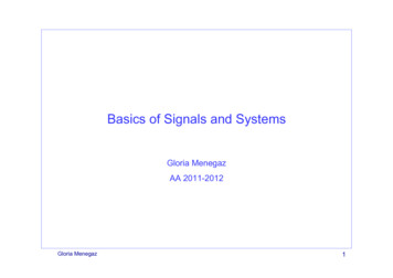
Illustration of the folding, displacement, and multiplicationsteps needed to perform two-dimensional x - α ,y - β)g(x - α ,y - β)(c)xα73(b)yBxβαβyVolume f(x,y) * g(x,y)(d)
Matrix perspectiveihgfedcbacbaabcfeddefihgghistep 2step 174
Convolution Exampleh1-1-112-1111Rotate111-121-1-11From C. Rasmussen, U. of Delaware75f2223213322121322
Convolution Example1112223-1212133-1-1122121322Step 1h111-124223-12-213322121322f765f*h
Convolution 33-1-112212132254f*h
Convolution 33-1-1122121322544f*h
Convolution 3-33-3122121322f544f*h-2
Convolution 39-1-222121322f44f*h-2
Convolution 3962-22-2121322f4f*h-2
Basics of Signals and Systems Gloria Menegaz AA 2011-2012 1 . Gloria Menegaz Didactic materia l Textbook – Signal Processing and Linear Systems, B.P. Lathi, CRC Press . – Real world signals (audio, E