WIXLIB

ML Cheatsheet Documentationdef normalize(features):**features(200, 3)features.T(3, 200)We transpose the input matrix, swappingcols and rows to make vector math easier**for feature in features.T:fmean np.mean(feature)frange np.amax(feature) - np.amin(feature)#Vector Subtractionfeature - fmean#Vector Divisionfeature / frangereturn featuresNote: Matrix math. Before we continue, it’s important to understand basic Linear Algebra concepts as well asnumpy functions like numpy.dot().1.3.3 Making predictionsOur predict function outputs an estimate of sales given our current weights (coefficients) and a company’s TV, radio,and newspaper spend. Our model will try to identify weight values that most reduce our cost function.𝑆𝑎𝑙𝑒𝑠 𝑊1 𝑇 𝑉 𝑊2 𝑅𝑎𝑑𝑖𝑜 𝑊3 𝑁 𝑒𝑤𝑠𝑝𝑎𝑝𝑒𝑟def predict(features, weights):**features - (200, 3)weights - (3, 1)predictions - (200,1)**predictions np.dot(features, weights)return predictions1.3.4 Initialize weightsW1 0.0W2 0.0W3 0.0weights np.array([[W1],[W2],[W3]])1.3. Multivariable regression15

ML Cheatsheet Documentation1.3.5 Cost functionNow we need a cost function to audit how our model is performing. The math is the same, except we swap the 𝑚𝑥 𝑏expression for 𝑊1 𝑥1 𝑊2 𝑥2 𝑊3 𝑥3 . We also divide the expression by 2 to make derivative calculations simpler.𝑀 𝑆𝐸 𝑛1 ︁(𝑦𝑖 (𝑊1 𝑥1 𝑊2 𝑥2 𝑊3 𝑥3 ))22𝑁 𝑖 1def cost function(features, targets, weights):**features:(200,3)targets: (200,1)weights:(3,1)returns average squared error among predictions**N len(targets)predictions predict(features, weights)# Matrix math lets use do this without loopingsq error (predictions - targets)**2# Return average squared error among predictionsreturn 1.0/(2*N) * sq error.sum()1.3.6 Gradient descentAgain using the Chain rule we can compute the gradient–a vector of partial derivatives describing the slope of the costfunction for each weight.𝑓 ′ (𝑊1 ) 𝑥1 (𝑦 (𝑊1 𝑥1 𝑊2 𝑥2 𝑊3 𝑥3 ))(1.3)𝑓 ′ (𝑊2 ) 𝑥2 (𝑦 (𝑊1 𝑥1 𝑊2 𝑥2 𝑊3(1.4)𝑥3 ))𝑓 ′ (𝑊3 ) 𝑥3 (𝑦 (𝑊1 𝑥1 𝑊2 𝑥2 𝑊3(1.5)𝑥3 ))def update weights(features, targets, weights, lr):'''Features:(200, 3)Targets: (200, 1)Weights:(3, 1)'''predictions predict(features, weights)#Extract our featuresx1 features[:,0]x2 features[:,1]x3 features[:,2]# Use dot product to calculate the derivative for each weightd w1 -x1.dot(targets - predictions)d w2 -x2.dot(targets - predictions)d w2 -x2.dot(targets - predictions)# Multiply the mean derivative by the learning rate(continues on next page)16Chapter 1. Linear Regression

ML Cheatsheet Documentation(continued from previous page)# and subtract from our weights (remember gradient points in direction of steepest ASCENT)weights[0][0] - (lr * np.mean(d w1))weights[1][0] - (lr * np.mean(d w2))weights[2][0] - (lr * np.mean(d w3))return weightsAnd that’s it! Multivariate linear regression.1.3.7 Simplifying with matricesThe gradient descent code above has a lot of duplication. Can we improve it somehow? One way to refactor would beto loop through our features and weights–allowing our function to handle any number of features. However there isanother even better technique: vectorized gradient descent.MathWe use the same formula as above, but instead of operating on a single feature at a time, we use matrix multiplicationto operative on all features and weights simultaneously. We replace the 𝑥𝑖 terms with a single feature matrix 𝑋.𝑔𝑟𝑎𝑑𝑖𝑒𝑛𝑡 𝑋(𝑡𝑎𝑟𝑔𝑒𝑡𝑠 𝑝𝑟𝑒𝑑𝑖𝑐𝑡𝑖𝑜𝑛𝑠)CodeX [[x1, x2, x3][x1, x2, x3].[x1, x2, x3]]targets [[1],[2],[3]]def update weights vectorized(X, targets, weights, lr):**gradient X.T * (predictions - targets) / NX: (200, 3)Targets: (200, 1)Weights: (3, 1)**companies len(X)#1 - Get Predictionspredictions predict(X, weights)(continues on next page)1.3. Multivariable regression17

ML Cheatsheet Documentation(continued from previous page)#2 - Calculate error/losserror targets - predictions#3 Transpose features from (200, 3) to (3, 200)# So we can multiply w the (200,1) error matrix.# Returns a (3,1) matrix holding 3 partial derivatives -# one for each feature -- representing the aggregate# slope of the cost function across all observationsgradient np.dot(-X.T, error)#4 Take the average error derivative for each featuregradient / companies#5 - Multiply the gradient by our learning rategradient * lr#6 - Subtract from our weights to minimize costweights - gradientreturn weights1.3.8 Bias termOur train function is the same as for simple linear regression, however we’re going to make one final tweak beforerunning: add a bias term to our feature matrix.In our example, it’s very unlikely that sales would be zero if companies stopped advertising. Possible reasons for thismight include past advertising, existing customer relationships, retail locations, and salespeople. A bias term will helpus capture this base case.CodeBelow we add a constant 1 to our features matrix. By setting this value to 1, it turns our bias term into a constant.bias np.ones(shape (len(features),1))features np.append(bias, features, axis 1)1.3.9 Model evaluationAfter training our model through 1000 iterations with a learning rate of .0005, we finally arrive at a set of weights wecan use to make predictions:𝑆𝑎𝑙𝑒𝑠 4.7𝑇 𝑉 3.5𝑅𝑎𝑑𝑖𝑜 .81𝑁 𝑒𝑤𝑠𝑝𝑎𝑝𝑒𝑟 13.9Our MSE cost dropped from 110.86 to 6.25.18Chapter 1. Linear Regression

ML Cheatsheet DocumentationReferences1.3. Multivariable regression19

ML Cheatsheet Documentation20Chapter 1. Linear Regression

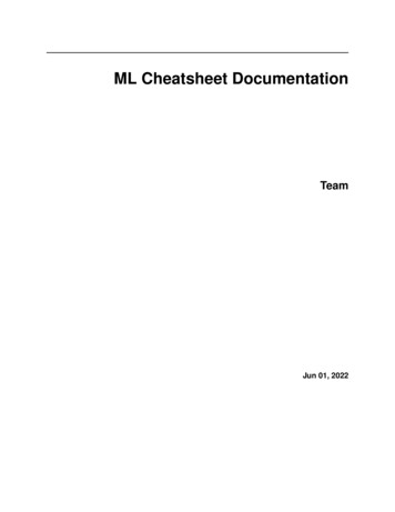
CHAPTER2Gradient DescentGradient descent is an optimization algorithm used to minimize some function by iteratively moving in the directionof steepest descent as defined by the negative of the gradient. In machine learning, we use gradient descent to updatethe parameters of our model. Parameters refer to coefficients in Linear Regression and weights in neural networks.2.1 IntroductionConsider the 3-dimensional graph below in the context of a cost function. Our goal is to move from the mountain inthe top right corner (high cost) to the dark blue sea in the bottom left (low cost). The arrows represent the direction ofsteepest descent (negative gradient) from any given point–the direction that decreases the cost function as quickly aspossible. SourceStarting at the top of the mountain, we take our first step downhill in the direction specified by the negative gradient.Next we recalculate the negative gradient (passing in the coordinates of our new point) and take another step in thedirection it specifies. We continue this process iteratively until we get to the bottom of our graph, or to a point wherewe can no longer move downhill–a local minimum. image source.21

ML Cheatsheet Documentation2.2 Learning rateThe size of these steps is called the learning rate. With a high learning rate we can cover more ground each step, butwe risk overshooting the lowest point since the slope of the hill is constantly changing. With a very low learning rate,we can confidently move in the direction of the negative gradient since we are recalculating it so frequently. A lowlearning rate is more precise, but calculating the gradient is time-consuming, so it will take us a very long time to getto the bottom.2.3 Cost functionA Loss Functions tells us “how good” our model is at making predictions for a given set of parameters. The costfunction has its own curve and its own gradients. The slope of this curve tells us how to update our parameters to makethe model more accurate.2.4 Step-by-stepNow let’s run gradient descent using our new cost function. There are two parameters in our cost function we cancontrol: 𝑚 (weight) and 𝑏 (bias). Since we need to consider the impact each one has on the final prediction, we needto use partial derivatives. We calculate the partial derivatives of the cost function with respect to each parameter andstore the results in a gradient.MathGiven the cost function:𝑓 (𝑚, 𝑏) 22𝑛1 ︁(𝑦𝑖 (𝑚𝑥𝑖 𝑏))2𝑁 𝑖 1Chapter 2. Gradient Descent

ML Cheatsheet DocumentationThe gradient can be calculated as:𝑓 ′ (𝑚, 𝑏) [︂𝑑𝑓𝑑𝑚𝑑𝑓𝑑𝑏]︂ ]︂[︂ 1 ︀𝑁 ︀ 2𝑥𝑖 (𝑦𝑖 (𝑚𝑥𝑖 𝑏))1 2(𝑦𝑖 (𝑚𝑥𝑖 𝑏))𝑁To solve for the gradient, we iterate through our data points using our new 𝑚 and 𝑏 values and compute the partialderivatives. This new gradient tells us the slope of our cost function at our current position (current parameter values)and the direction we should move to update our parameters. The size of our update is controlled by the learning rate.Codedef update weights(m, b, X, Y, learning rate):m deriv 0b deriv 0N len(X)for i in range(N):# Calculate partial derivatives# -2x(y - (mx b))m deriv -2*X[i] * (Y[i] - (m*X[i] b))# -2(y - (mx b))b deriv -2*(Y[i] - (m*X[i] b))# We subtract because the derivatives point in direction of steepest ascentm - (m deriv / float(N)) * learning rateb - (b deriv / float(N)) * learning ratereturn m, bReferences2.4. Step-by-step23

ML Cheatsheet Documentation24Chapter 2. Gradient Descent

CHAPTER3Logistic Regression Introduction– Comparison to linear regression– Types of logistic regression Binary logistic regression– Sigmoid activation– Decision boundary– Making predictions– Cost function– Gradient descent– Mapping probabilities to classes– Training– Model evaluation Multiclass logistic regression– Procedure– Softmax activation– Scikit-Learn example3.1 IntroductionLogistic regression is a classification algorithm used to assign observations to a discrete set of classes. Unlike linearregression which outputs continuous number values, logistic regression transforms its output using the logistic sigmoid25

ML Cheatsheet Documentationfunction to return a probability value which can then be mapped to two or more discrete classes.3.1.1 Comparison to linear regressionGiven data on time spent studying and exam scores. Linear Regression and logistic regression can predict differentthings: Linear Regression could help us predict the student’s test score on a scale of 0 - 100. Linear regressionpredictions are continuous (numbers in a range). Logistic Regression could help use predict whether the student passed or failed. Logistic regression predictionsare discrete (only specific values or categories are allowed). We can also view probability scores underlying themodel’s classifications.3.1.2 Types of logistic regression Binary (Pass/Fail) Multi (Cats, Dogs, Sheep) Ordinal (Low, Medium, High)3.2 Binary logistic regressionSay we’re given data on student exam results and our goal is to predict whether a student will pass or fail based onnumber of hours slept and hours spent studying. We have two features (hours slept, hours studied) and two classes:passed (1) and failed ssed1010Graphically we could represent our data with a scatter plot.26Chapter 3. Logistic Regression

ML Cheatsheet Documentation3.2.1 Sigmoid activationIn order to map predicted values to probabilities, we use the sigmoid function. The function maps any real value intoanother value between 0 and 1. In machine learning, we use sigmoid to map predictions to probabilities.Math𝑆(𝑧) 11 𝑒 𝑧Note: 𝑠(𝑧) output between 0 and 1 (probability estimate) 𝑧 input to the function (your algorithm’s prediction e.g. mx b) 𝑒 base of natural log3.2. Binary logistic regression27

ML Cheatsheet DocumentationGraphCodedef sigmoid(z):return 1.0 / (1 np.exp(-z))3.2.2 Decision boundaryOur current prediction function returns a probability score between 0 and 1. In order to map this to a discrete class(true/false, cat/dog), we select a threshold value or tipping point above which we will classify values into class 1 andbelow which we classify values into class 2.𝑝 0.5, 𝑐𝑙𝑎𝑠𝑠 1𝑝 0.5, 𝑐𝑙𝑎𝑠𝑠 028Chapter 3. Logistic Regression

ML Cheatsheet DocumentationFor example, if our threshold was .5 and our prediction function returned .7, we would classify this observation aspositive. If our prediction was .2 we would classify the observation as negative. For logistic regression with multipleclasses we could select the class with the highest predicted probability.3.2.3 Making predictionsUsing our knowledge of sigmoid functions and decision boundaries, we can now write a prediction function. Aprediction function in logistic regression returns the probability of our observation being positive, True, or “Yes”. Wecall this class 1 and its notation is 𝑃 (𝑐𝑙𝑎𝑠𝑠 1). As the probability gets closer to 1, our model is more confident thatthe observation is in class 1.MathLet’s use the same multiple linear regression equation from our linear regression tutorial.𝑧 𝑊0 𝑊1 𝑆𝑡𝑢𝑑𝑖𝑒𝑑 𝑊2 𝑆𝑙𝑒𝑝𝑡This time however we will transform the output using the sigmoid function to return a probability value between 0 and1.𝑃 (𝑐𝑙𝑎𝑠𝑠 1) 11 𝑒 𝑧If the model returns .4 it believes there is only a 40% chance of passing. If our decision boundary was .5, we wouldcategorize this observation as “Fail.””CodeWe wrap the sigmoid function over the same prediction function we used in multiple linear regression3.2. Binary logistic regression29

ML Cheatsheet Documentationdef predict(features, weights):'''Returns 1D array of probabilitiesthat the class label 1'''z np.dot(features, weights)return sigmoid(z)3.2.4 Cost functionUnfortunately we can’t (or at least shouldn’t) use the same cost function MSE (L2) as we did for linear regression.Why? There is a great math explanation in chapter 3 of Michael Neilson’s deep learning book5 , but for now I’ll simplysay it’s because our prediction function is non-linear (due to sigmoid transform). Squaring this prediction as we doin MSE results in a non-convex function with many local minimums. If our cost function has many local minimums,gradient descent may not find the optimal global minimum.MathInstead of Mean Squared Error, we use a cost function called Cross-Entropy, also known as Log Loss. Cross-entropyloss can be divided into two separate cost functions: one for 𝑦 1 and one for 𝑦 0.The benefits of taking the logarithm reveal themselves when you look at the cost function graphs for y 1 and y 0.These smooth monotonic functions7 (always increasing or always decreasing) make it easy to calculate the gradientand minimize cost. Image from Andrew Ng’s slides on logistic regression1 onic functionhttp://www.holehouse.org/mlclass/06 Logistic Regression.htmlChapter 3. Logistic Regression

ML Cheatsheet DocumentationThe key thing to note is the cost function penalizes confident and wrong predictions more than it rewards confidentand right predictions! The corollary is increasing prediction accuracy (closer to 0 or 1) has diminishing returns onreducing cost due to the logistic nature of our cost function.Above functions compressed into oneMultiplying by 𝑦 and (1 𝑦) in the above equation is a sneaky trick that let’s us use the same equation to solve forboth y 1 and y 0 cases. If y 0, the first side cancels out. If y 1, the second side cancels out. In both cases we onlyperform the operation we need to perform.Vectorized cost functionCodedef cost function(features, labels, weights):'''Using Mean Absolute ErrorFeatures:(100,3)Labels: (100,1)Weights:(3,1)(continues on next page)3.2. Binary logistic regression31

ML Cheatsheet Documentation(continued from previous page)Returns 1D matrix of predictionsCost (labels*log(predictions) (1-labels)*log(1-predictions) ) / len(labels)'''observations len(labels)predictions predict(features, weights)#Take the error when label 1class1 cost -labels*np.log(predictions)#Take the error when label 0class2 cost (1-labels)*np.log(1-predictions)#Take the sum of both costscost class1 cost - class2 cost#Take the average costcost cost.sum() / observationsreturn cost3.2.5 Gradient descentTo minimize our cost, we use Gradient Descent just like before in Linear Regression. There are other more sophisticated optimization algorithms out there such as conjugate gradient like BFGS, but you don’t have to worry about these.Machine learning libraries like Scikit-learn hide their implementations so you can focus on more interesting things!MathOne of the neat properties of the sigmoid function is its derivative is easy to calculate. If you’re curious, there is agood walk-through derivation on stack overflow6 . Michael Neilson also covers the topic in chapter 3 of his book.𝑠′ (𝑧) 𝑠(𝑧)(1 𝑠(𝑧))(3.1)Which leads to an equally beautiful and convenient cost function derivative:𝐶 ′ 𝑥(𝑠(𝑧) 𝑦)Note: 𝐶 ′ is the derivative of cost with respect to weights 𝑦 is the actual class label (0 or 1) 𝑠(𝑧) is your model’s prediction 𝑥 is your feature or feature vector.Notice how this gradient is the same as the MSE (L2) gradient, the only difference is the hypothesis c11e-xChapter 3. Logistic Regression

ML Cheatsheet DocumentationPseudocodeRepeat {1. Calculate gradient average2. Multiply by learning rate3. Subtract from weights}Codedef update weights(features, labels, weights, lr):'''Vectorized Gradient DescentFeatures:(200, 3)Labels: (200, 1)Weights:(3, 1)'''N len(features)#1 - Get Predictionspredictions predict(features, weights)#2 Transpose features from (200, 3) to (3, 200)# So we can multiply w the (200,1) cost matrix.# Returns a (3,1) matrix holding 3 partial derivatives -# one for each feature -- representing the aggregate# slope of the cost function across all observationsgradient np.dot(features.T, predictions - labels)#3 Take the average cost derivative for each featuregradient / N#4 - Multiply the gradient by our learning rategradient * lr#5 - Subtract from our weights to minimize costweights - gradientreturn weights3.2.6 Mapping probabilities to classesThe final step is assign class labels (0 or 1) to our predicted probabilities.Decision boundarydef decision boundary(prob):return 1 if prob .5 else 03.2. Binary logistic regression33

ML Cheatsheet DocumentationConvert probabilities to classesdef classify(predictions):'''input - N element array of predictions between 0 and 1output - N element array of 0s (False) and 1s (True)'''decision boundary np.vectorize(decision boundary)return decision boundary(predictions).flatten()Example outputProbabilities [ 0.967, 0.448, 0.015, 0.780, 0.978, 0.004]Classifications [1, 0, 0, 1, 1, 0]3.2.7 TrainingOur training code is the same as we used for linear regression.def train(features, labels, weights, lr, iters):cost history []for i in range(iters):weights update weights(features, labels, weights, lr)#Calculate error for auditing purposescost cost function(features, labels, weights)cost history.append(cost)# Log Progressif i % 1000 0:print "iter: " str(i) " cost: " str(cost)return weights, cost history3.2.8 Model evaluationIf our model is working, we should see our cost decrease after every iteration.iter: 0 cost: 0.635iter: 1000 cost: 0.302iter: 2000 cost: 0.264Final cost: 0.2487. Final weights: [-8.197, .921, .738]34Chapter 3. Logistic Regression

ML Cheatsheet DocumentationCost historyAccuracyAccuracy measures how correct our predictions were. In this case we simply compare predicted labels to true labelsand divide by the total.def accuracy(predicted labels, actual labe

22 Reinforcement Learning 165 23 Datasets 169 24 Libraries 185 25 Papers 215 26 Other Content 221 27 Contribute 227 ii. ML Cheatsheet Documentation Brief visual explanations of machine learning concepts with diagrams, code examples and links to resources for learning more.