Transcription
An Advanced Guide toTrade Policy Analysis:The Structural Gravity ModelYoto V. Yotov,Roberta Piermartini,José-Antonio Monteiro,and Mario Larch
What is An Advanced Guide to Trade Policy Analysis?An Advanced Guide to Trade Policy Analysis aims to helpresearchers and policymakers update their knowledge ofquantitative economic methods and data sources for tradepolicy analysis.Using this guideThe guide explains analytical techniques, reviews the datanecessary for analysis and includes illustrative applicationsand exercises.Find out moreWebsite: http://vi.unctad.org/tpa
An Advanced Guide toTrade Policy Analysis:The Structural Gravity Model
ction5A. The gravity model: a workhorse of applied internationaltrade analysis5B. Using this guide6CHAPTER 1: PARTIAL EQUILIBRIUM TRADE POLICYANALYSIS WITH STRUCTURAL GRAVITY9A. Overview and learning objectives11B. Analytical tools121. Structural gravity: from theory to empirics122. Gravity estimation: challenges, solutions andbest practices173. Gravity estimates: interpretation and aggregation284. Gravity data: sources and limitations32C. Applications401. Traditional gravity estimates412. The “distance puzzle” resolved453. Regional trade agreements effects49D. Exercises551. Estimating the effects of the WTO accession552. Estimating the effects of unilateral trade policy561
AppendicesAppendix A: Structural gravity from supply side57Appendix B: Structural gravity with tariffs60Appendix C: Databases and data sources links summary63Chapter 2: General equilibrium trade policy analysis withstructural gravity67A. Overview and learning objectives69B. Analytical tools701. Structural gravity: general equilibrium context702. Standard approach to general equilibrium analysiswith structural gravity883. A general equilibrium gravity analysis with the PoissonPseudo Maximum Likelihood (GEPPML)95C. Applications1021. Trade without borders1032. Impact of regional trade agreements111D. Exercises1171. Calculating the general equilibrium impacts ofremoving a specific border1172. Calculating the general equilibrium impacts of aregional trade agreement118Appendices119Appendix A: Counterfactual analysis usingsupply-side gravity framework119Appendix B: Structural gravity with sectors121Appendix C: Structural gravity system in changes126References257131
AUTHORSYoto V. YotovDrexel University, CESifo and ERI-BASRoberta PiermartiniEconomic Research and Statistics Division, World Trade OrganizationJosé-Antonio MonteiroEconomic Research and Statistics Division, World Trade OrganizationMario LarchUniversity of Bayreuth, CESifo, ifo Institute, and GEP at University of NottinghamAcknowledgmentsThe authors would like to thank Michela Esposito for her comments and valuable researchassistance. They also would like to thank Delina Agnosteva, James Anderson, Richard Barnett,Davin Chor, Gabriel Felbermayr, Benedikt Heid, Russell Hillberry, Lou Jing, Ma Lin, AntonellaLiberatore, Andreas Maurer, Jurgen Richtering, Stela Rubinova, Serge Shikher, CostasSyropoulos, Robert Teh, Thomas Verbeet, Mykyta Vesselovsky, Joschka Wanner, ThomasZylkin, as well as the seminar and workshop participants at the ifo Institute, the World TradeOrganization, the World Bank, the U.S. International Trade Commission, Global Affairs Canada,the University of Ottawa, the Kiel Institute for the World Economy, the Tsenov Academy ofEconomics, and the National University of Singapore for helpful suggestions and discussions.Thanks also go to Vlasta Macku (UNCTAD Virtual Institute) for her continuous support to thisproject and her role in initiating this inter-organizational cooperation.The production of this book was managed by WTO Publications. Anthony Martin has edited thetext. The website was developed by Susana Olivares.3
DISCLAIMERThe designations employed in UNCTAD and WTO publications, which are in conformity withUnited Nations practice, and the presentation of material therein do not imply the expression ofany opinion whatsoever on the part of the United Nations Conference on Trade and Developmentor the World Trade Organization concerning the legal status of any country, area or territory orof its authorities, or concerning the delimitation of its frontiers. The responsibility for opinionsexpressed in studies and other contributions rests solely with their authors, and publication doesnot constitute an endorsement by the United Nations Conference on Trade and Developmentor the World Trade Organization of the opinions expressed. Reference to names of firms andcommercial products and processes does not imply their endorsement by the United NationsConference on Trade and Development or the World Trade Organization, and any failure to mentiona particular firm, commercial product or process is not a sign of disapproval.4
INTRODUCTIONA. The gravity model: a workhorse of appliedinternational trade analysisQuantitative and detailed trade policy information and analysis are more necessary now than theyhave ever been. In recent years, globalization and, more specifically, trade opening have becomeincreasingly contentious. It is, therefore, important for policy-makers and other trade policy stakeholders to have access to detailed, reliable information and analysis on the effects of trade policies,as this information is needed at different stages of the policy-making process.Often referred to as the workhorse in international trade, the gravity model is one of the mostpopular and successful frameworks in economics. Hundreds of papers have used the gravityequation to study and quantify the effects of various determinants of international trade. Thereare at least five compelling arguments that, in combination, may explain the remarkable successand popularity of the gravity model. First, the gravity model of trade is very intuitive. Using the metaphor of Newton’sLaw of Universal Gravitation, the gravity model of trade predicts that international trade(gravitational force) between two countries (objects) is directly proportional to the productof their sizes (masses) and inversely proportional to the trade frictions (the square ofdistance) between them. Second, the gravity model of trade is a structural model with solid theoretical foundations.This property makes the gravity framework particularly appropriate for counterfactual analysis,such as quantifying the effects of trade policy. Third, the gravity model represents a realistic general equilibrium environment thatsimultaneously accommodates multiple countries, multiple sectors, and even firms. As such,the gravity framework can be used to capture the possibility that markets (sectors, countries,etc.) are linked and that trade policy changes in one market will trigger ripple effects in therest of the world. Fourth, the gravity setting is a very flexible structure that can be integrated within a wideclass of broader general equilibrium models in order to study the links between trade andlabour markets, investment, the environment, etc. Finally, one of the most attractive properties of the gravity model is its predictive power.Empirical gravity equations of trade flows consistently deliver a remarkable fit of between60 and 90 percent with aggregate data as well as with sectoral data for both goods andservices.15
AN ADVANCED GUIDE TO TRADE POLICY ANALYSISCapitalizing on the appealing properties of the gravity model, this Advanced Guide to Trade PolicyAnalysis complements and is best used in conjunction with the Practical Guide to Trade Policy Analysispublished in 2012. In particular, the Advanced Guide presented in Chapter 3 a brief overview ofthe theoretical foundation of gravity models, possible estimation methods, and advanced modellingissues, such as the handling of zero-trade flows and calculation of tariff equivalents of non-tariffbarriers. The Practical Guide also discussed data sources for gravity analysis and explains how tobuild a gravity database.Chapter 1 of this Advanced Guide reconsiders some of these issues, including data challenges andsources, but also integrates the latest developments in the empirical gravity literature by proposingsix recommendations to obtain reliable estimates of the partial equilibrium effects of bilateraland non-discriminatory trade policies within the same comprehensive, and theoretically-consistenteconometric specification of the structural gravity model.In addition, unlike the Practical Guide, which only presented in Chapter 5 what ComputableGeneral Equilibrium models are and when they should be used, Chapter 2 of this Advanced Guideoffers a deep analysis of the structural relationships underlying the general equilibrium gravitysystem, and how they can be exploited to make trade policy inferences. In particular, Chapter 2presents standard procedures to perform counterfactual analysis with the structural gravity modeland outlines the latest methods developed in the literature to obtain theory-consistent generalequilibrium effects of trade policy with a simple procedure that can be performed in moststatistical software packages. Chapter 2 further shows how the structural gravity model presentedin this Advanced Guide can be integrated within a larger class of general equilibrium models, suchas a dynamic gravity model.B. Using this GuideThis Advanced Guide is targeted at economists with advanced training and experience in appliedresearch and analysis. In particular, on the economics side, advanced knowledge of internationaltrade theory and policy is required, while on the empirical side, the prerequisite is familiarity withwork on databases and with the use of STATA software. The reader with limited experience withSTATA may wish to first review the applications and complete the exercises proposed in thePractical Guide to Trade Policy Analysis.The Guide comprises two chapters. Both chapters start with a brief introduction providing anoverview of the contents and setting out the learning objectives. Each chapter is further dividedinto two main parts. The first part introduces a number of theoretical concepts and analytical tools,and explains their economic logic. The first part of Chapter 1 also includes a discussion on datasources. The second part of both chapters describes how the analytical tools can be applied inpractice, showing how data can be processed to analyse the effects of the trade policies on tradeflows output, expenditures, real GDP and welfare. Each of these applications has been designedonly for a pedagogical purpose.6
IntroductionThe software used for partial and general equilibrium analysis with the structural gravity model isSTATA software. While the presentation of these applications in the chapters can stand alone,the files with the corresponding STATA commands and the relevant data can be found on thePractical Guide to Trade Policy Analysis website: http://vi.unctad.org/tpa. A general folder entitled“Advanced Guide to Trade Policy Analysis” is divided into sub-folders which correspond to eachchapter (e.g. “Advanced Guide to Trade Policy Analysis\Chapter1”). Within each of these subfolders, the reader will find datasets, applications and exercises. Detailed explanations can be foundin the file “readme.pdf” available on the website.Endnote1Head and Mayer (2014) offer representative estimates and evidence for the empirical success of gravitywith aggregate data. Anderson and Yotov (2010) present and discuss sectoral gravity estimates withgoods trade. Anderson et al. (2015a) demonstrate that gravity works very well with services sectoraldata. Finally, Aichele et al. (2014) estimate sectoral gravity for agriculture, mining, manufacturing goodsand services.7
CHAPTER 1CHAPTER 1: Partial equilibrium trade policy analysiswith structural gravity1TABLE OF CONTENTSA.Overview and learning objectives11B.Analytical tools1. Structural gravity: from theory to empirics2. Gravity estimation: challenges, solutions and best practices3. Gravity estimates: interpretation and aggregation4. Gravity data: sources and limitations1212172832C.Applications1. Traditional gravity estimates2. The “distance puzzle” resolved3. Regional trade agreements effects40414549D.Exercises1. Estimating the effects of WTO accession2. Estimating the effects of unilateral trade policy555556AppendicesAppendix A: Structural gravity from supply sideAppendix B: Structural gravity with tariffsAppendix C: Databases and data sources links summary57576063Endnotes659
LIST OF FIGURESFigure 1Gravity model’s strong theoretical foundations12LIST OF TABLESTable 1Table 2Table 3Traditional gravity estimatesA simple solution of the “distance puzzle” in tradeEstimating the effects of regional trade agreements424751LIST OF BOXESBox 1Box 210Analogy between the Newtonian theory of gravitation and gravitytrade modelIn the absence of panel trade data1726
CHAPTER 1: PARTIAL EQUILIBRIUM TRADE POLICY ANALYSIS WITH STRUCTURAL GRAVITYCHAPTER 1A. Overview and learning objectivesDespite solid theoretical foundations and remarkable empirical success, the empirical gravity equationis still often applied a-theoretically and without account for important estimation challenges that maylead to biased and even inconsistent gravity estimates. The objective of this chapter is to serve as apractical guide for estimating the effects of trade policies (and other determinants of bilateral trade)with the structural gravity model.The first part of this chapter will present a brief overview of the evolution of gravity theory over time and review the theoretical foundations of the Armington-Constant Elasticity ofSubstitution (CES) version of the structural gravity model. Importantly, the Armington-CESframework is used as a representative theoretical setting for a wide family of trade models thatall lead to the same empirical gravity specification. Next, the main challenges faced when estimating the gravity model will be discussed along with the solutions that have been proposedin the trade literature to address them. Drawing from the latest developments in the empiricalgravity literature, six recommendations will be formulated to obtain reliable partial equilibriumestimates of the effects of bilateral and non-discriminatory trade policies within the same comprehensive and theoretically-consistent econometric specification. Interpretation of the partialequilibrium gravity estimates and methods to consistently aggregate bilateral trade costs willthen be discussed. Finally, data sources for gravity analysis, including bilateral trade flows andtrade costs, will be provided.Once familiarized with these theoretical concepts and analytical tools, a series of empirical applications, demonstrating the usefulness, validity and applicability of the recommendations proposedwill be presented. Specifically, instructions will be provided on how to estimate a structural gravitymodel in order to assess the partial equilibrium effects of traditional gravity variables (e.g. distance,common language ), globalization, and regional trade agreements (RTAs) (as a representativeform of bilateral trade policy).Two exercises are provided at the end of the chapter. Data and STATA do-files for the solution ofthese exercises can be downloaded from the website.In this chapter, you will learn: How the structural gravity model is derived; Where to find the data needed to estimate econometrically the structural gravity model; What are the main measurement issues associated with gravity data; What are the main econometric issues associated with the estimation of the structural gravitymodel and how to address them; How to econometrically estimate the structural gravity model; How to interpret and consistently aggregate gravity estimates.11
AN ADVANCED GUIDE TO TRADE POLICY ANALYSISAfter reading this chapter, with good econometric knowledge, and familiarity with STATA, you willbe able to estimate using STATA software a theoretically-consistent structural gravity model andassess the effects of trade policies (and other determinants) on bilateral trade, while interpretingthe econometric results with key caveats in mind.B. Analytical tools1. Structural gravity: from theory to empirics(a) Evolution of gravity theory over timeAccording to Newton’s Law of Universal Gravitation, any particle in the universe attracts anyother particle thanks to a force that is directly proportional to the product of their masses andinversely proportional to the square of the distance between them. Applied to international trade,Newton’s Law of Gravity implies that, just as particles are mutually attracted in proportion totheir sizes and proximity, countries trade in proportion to their respective market size (e.g. grossdomestic products) and proximity.The initial applications of Newton’s Law of Gravitation to economics are a-theoretical. Prominentexamples include Ravenstein (1885) and Tinbergen (1962), who used gravity to study immigrationand trade flows, respectively. Anderson (1979) is the first to offer a theoretical economic foundation for the gravity equation under the assumptions of product differentiation by place of origin andConstant Elasticity of Substitution (CES) expenditures. Another early contribution to gravity theoryis Bergstrand (1985).Despite these theoretical developments and its solid empirical performance, the gravity model oftrade struggled to make much impact in the profession until the late 1990s and early 2000s.Arguably, the most influential structural gravity theories in economics are those of Eaton andFigure 1Gravity model’s strong theoretical foundationsArmington-CESDynamics andFactor nopolisticCompetitionGravitySectoral 12Ricardian
CHAPTER 1: PARTIAL EQUILIBRIUM TRADE POLICY ANALYSIS WITH STRUCTURAL GRAVITYCHAPTER 1Kortum (EK) (2002), who derived gravity on the supply side as a Ricardian structure with intermediate goods, and Anderson and van Wincoop (2003), who popularized the Armington-CES model ofAnderson (1979) and emphasized the importance of the general equilibrium effects of trade costs.The academic interest in the gravity model was recently stimulated by the influential work ofArkolakis et al. (2012), who demonstrated that a large class of models generate isomorphicgravity equations which preserves the gains from trade. As depicted in Figure 1, the gainsfrom trade are invariant to a series of alternative micro-foundations including a single economymodel with monopolistic competition (Anderson, 1979; Anderson and van Wincoop, 2003);a Heckscher-Ohlin framework (Bergstrand, 1985; Deardoff, 1998); a Ricardian framework(Eaton and Kortum, 2002); entry of heterogeneous firms, selection into markets (Chaney, 2008;Helpman et al., 2008); a sectoral Armington-model (Anderson and Yotov, 2016); a sectoralRicardian model (Costinot et al., 2012; Chor, 2010); a sectoral input-output linkages gravitymodel based on Eaton and Kortum (2002) (Caliendo and Parro, 2015), and a dynamic framework with asset accumulation (Olivero and Yotov, 2012, Anderson et al. 2015C, and Eaton et al.,2016). Most recently, Allen et al. (2014) established the universal power of gravity by derivingsufficient conditions for the existence and uniqueness of the trade equilibrium for a wide classof general equilibrium trade models.(b) Review of the structural gravity modelOne of the main advantages of the structural gravity model is that it delivers a tractable framework fortrade policy analysis in a multi-country environment. Accordingly, the model reviewed in this AdvancedGuide considers a world that consists of N countries, where each economy produces a variety ofgoods (i.e. goods are differentiated by place of origin (Armington, 1969)) that is traded with the restof the world. The supply of each good is fixed to Qi , and the factory-gate price for each variety is pi .Thus, the value of domestic production in a representative economy is defined as Yi pi Qi , where Yiis also the nominal income in country i. Country i’s aggregate expenditure is denoted by Ei . Aggregateexpenditure can also be expressed in terms of nominal income by Ei φiYi , where φi 1 shows thatcountry i runs a trade deficit, while 1 φi 0 reflects a trade surplus. Similar to Dekle et al. (2007;2008), trade deficits and surpluses are treated as exogenous. For brevity’s sake, the time dimension tis omitted in the derivation of the structural gravity model. In addition, the structural gravity model presented below is derived from the demand side. However, as demonstrated in Appendix A, the samegravity system can be derived from the supply side.On the demand side, consumer preferences are assumed to be homothetic, identical across countries,and given by a CES-utility function for country j:2σ1 σ σ 1 σ 1 αi σ cij σ i (1-1)where σ 1 is the elasticity of substitution among different varieties, i.e. goods from differentcountries, αi 0 is the CES preference parameter, which will remain treated as an exogenoustaste parameter and cij denotes consumption of varieties from country i in country j.13
AN ADVANCED GUIDE TO TRADE POLICY ANALYSISConsumers maximize equation (1-1) subject to the following standard budget constraint: pij ciji Ej(1-2)Equation (1-2) ensures that the total expenditure in country j, Ej , is equal to the total spending onvarieties from all countries, including j, at delivered prices pij pitij , which are defined convenientlyas a function of factory-gate prices in the country of origin, pi , marked up by bilateral trade costs,tij 1, between trading partners i and j. Throughout the analysis, the bilateral trade costs aredefined as iceberg costs, as is standard in the trade literature (Samuelson, 1952). In order todeliver one unit of its variety to country j, country i must ship tij 1 units, i.e. 1/tij of the initialshipment melts “en route”. While the Armington model presumes that all bilateral trade costs arevariable, in principle, structural gravity can also accommodate fixed trade costs (Melitz, 2003).The iceberg trade costs metaphor can also be extended to accommodate fixed costs withthe interpretation that “a chunk of the iceberg breaks off as it parts from the mother glacier”(Anderson, 2011).Solving the consumer’s optimization problem yields the expenditures on goods shipped from origini to destination j as:3 αi pit ijXij Pj (1 σ )Ej(1-3)where Xij denotes trade flows from exporter i to destination j and, for now, Pi can be interpreted asa CES consumer price index: Pj αi pit ij i(11 σ 1 σ) (1-4)Given that the elasticity of substitution is greater than one, σ 1, equation (1-3) captures severalintuitive relationships. In particular, expenditure in country j on goods from source i, Xij , is:(i) proportional to total expenditure, Ej , in destination j. The simple intuition is that, all else equal,larger/richer markets consume more of all varieties, including goods from i.(ii) inversely related to the (delivered) prices of varieties from origin i to destination j, pij pitij . Thisis a direct reflection of the law of demand, which depends not only on factory-gate price pibut also on bilateral trade cost tij between partners i and j. The ideal combination that favoursbilateral trade is an efficient producer, characterized by low factory-gate price, and low bilateraltrade cost between countries i and j.14
CHAPTER 1: PARTIAL EQUILIBRIUM TRADE POLICY ANALYSIS WITH STRUCTURAL GRAVITYCHAPTER 1(iii) directly related to the CES price aggregator Pj . This relationship reflects the substitutioneffects across varieties from different countries. All else equal, the relatively more expensivethe rest of the varieties in the world are, the more consumers in country j will substitute awayfrom them and toward the goods from country i.(iv) contingent on the elasticity of substitution σi when factory-gate prices or the aggregate CES prices(or in the combination of those as a relative price) change. All else equal, a higher elasticity ofsubstitution will magnify the trade diversion effects from the more expensive commodities to thecheaper ones.The final step in the derivation of the structural gravity model is to impose market clearance forgoods from each origin: αi pit ij Pj Yi j1 σ (1-5)EjEquation (1-5) states that, at delivered prices (because part of the shipments melt “en route”), thevalue of output in country i, Yi , should be equal to the total expenditure of this country’s variety in allcountries in the world, including i itself. To see this intuition more clearly, note that the right-handside expression in equation (1-5) can be replaced with the sum of all bilateral shipments from i asdefined in equation (1-3), so that Yi j Xij j .Defining Y iYi and dividing equation (1-5) by Y, the terms can be rearranged to obtain:1 σ(αi pi ) YiY t ij Pj j1 σ (1-6)EjYFollowing Anderson and van Wincoop (2003), the term in the denominator of equation (1-6) can1 σE j Y , and be substituted into equation (1-6):be defined as Π1i σ j t ij Pj((αi pi )1 σ Yi Y)(1-7)Π1i σUsing equation (1-7) to substitute for the power transform (αi pi )1-σ in equations (1-3) and(1-4), and combining the definition of Π1i σ with the resulting expressions that correspond toequations (1-3) and (1-4), the structural gravity system is given by:1 σXij Yi E j t ij Y Πi Pj (1-8)15
AN ADVANCED GUIDE TO TRADE POLICY ANALYSIS1 σΠi t ij j PjEj(1-9)Y1 σ t ij Πi Pj1 σ i1 σ YiY(1-10)(c) Structural decomposition of gravity: size vs. trade costEquation (1-8), representing the theoretical gravity equation that governs bilateral trade flows,can be conveniently decomposed into two terms: (i) a size term, Yi Ej /Y, and a trade cost term,1 σt ij Πi Pj:( ((i)))The intuitive interpretation of the size term, Yi Ej /Y, is as the hypothetical level of frictionlesstrade between partners i and j if there were no trade costs.4 Mechanically, this can be shownby eliminating bilateral trade frictions (i.e. setting tij 1), and re-deriving the gravity system.Intuitively, a frictionless world implies that consumers will face the same price for a givenvariety regardless of their physical location and that their expenditure share on goods from aparticular country will be equal to the share of production in the source country in the globaleconomy (i.e. Xij /Ej Yi /Y ). Overall, the size term already carries some very useful informationregarding the relationship between country size and bilateral trade flows:5 namely, large producers will export more to all destinations; big/rich markets will import more from all sources;and trade flows between countries i and j will be larger the more similar in size the tradingpartners are.()1 σ(ii) The natural interpretation of the trade cost term, t ij ( Πi Pj ), is that it captures the totaleffects of trade costs that drive a wedge between realized and frictionless trade. The tradecost term consists of three components:(1) Bilateral trade cost between partners i and j, tij , is typically approximated in the literatureby various geographic and trade policy variables, such as bilateral distance, tariffs and thepresence of regional trade agreements (RTAs) between partners i and j.(2) The structural term Pj , coined by Anderson and van Wincoop (2003) as inward multilateralresistance represents importer j’s ease of market access.(3) The structural term Πi , defined as outward multilateral resistances by Anderson and vanWincoop (2003), measures exporter i’s ease of market access.As will be discussed in more details in section B.1 of Chapter 2, the multilateral resistances arethe vehicles that translate the initial, partial equilibrium effects of trade policy at the bilateral levelto country-specific effects on consumer and producer prices. The direct effects do give the initialimpact effects of trade costs on trade flows, while the general equilibrium trade costs also takeinto account the changes in prices, incomes and expenditures induced by trade cost changes.While this chapter focuses on the direct, partial effects of trade costs, chapter 2 deals with thegeneral equilibrium trade costs.16
CHAPTER 1: PARTIAL EQUILIBRIUM TRADE POLICY ANALYSIS WITH STRUCTURAL GRAVITYCHAPTER 1Box 1 Analogy between the Newtonian theory of gravitation and thegravity trade modelTo see the remarkable resemblance between the trade gravity equation and the correspondingequation from physics, two terms, Tijθ and G have to be defined in equation (1-8) as reportedin the right-hand side of the table below.Newton’s Law of Universal GravitationFij GMi M jDij2Gravity Trade ModelXij G where:where: Fij : gravitational force between objects i and jG: gravitational constantMi : object i ’s massMj: object j ’s massDij : distance between objects i and jYi E jTij θXij : exports from countries i and jG : inverse of world production G 1/ YYi : country i ’s domestic productionEj : country j ’s aggregate expenditureTijθ : total trade costs between countries i and j( ( Π P ))Tijθ t ijσ 1i jBased on the metaphor of Newton’s Law of Universal Gravitation, the gravity model of tradepredicts that international trade (gravitational force) between two countries (objects) is directlyproportional to the product of their sizes (masses) and inversely proportional to the trade frictions(the square of distance) between them.2. Gravity estimation: challenges, solutions and best practicesGiven the multiplicative nature of the structural gravity equation (1-8), and assuming that it holds ineach period of time t, it is possible to log-linearize it and expand it with an additive error term, εij,t :ln X ij ,t lnE j ,t lnYi ,t lnYt (1 σ )lnt ij ,t (1 σ )ln Pj ,t (1 σ )ln Π i ,t ε ij ,t(1-11)Specification (1-11) is the most popular version of the empir
"Advanced Guide to Trade Policy Analysis" is divided into sub-folders which correspond to each chapter (e.g. "Advanced Guide to Trade Policy Analysis\Chapter1"). Within each of these sub-folders, the reader will find datasets, applications and exercises. Detailed explanations can be found in the file "readme.pdf" available on the .